Lecture - Fundamental Concepts
Requisitos de conclusão
4. Receiver Response
4.1. Heterodyne frequency conversion
The detectors of radio telescopes are diodes with quadratic current-voltage characteristics that require an input power of  to work in the quadratic regime. The power
  of the weak radio-astronomical signals entering the receiver is given by
to work in the quadratic regime. The power of the weak radio-astronomical signals entering the receiver is given by
in which  is the Boltzmann constant and
  is the system temperature containing the receiver noise temperature and the antenna temperature. The antenna temperature is composed of the desired astronomical signal, a contribution from the earth's atmosphere, and possibly radiation from the ground. Due to that always present background the best case for the systemtemperature is
  . Therefore, using a typical bandwidth of
  , the input power
  , meaning that the signal must be amplified by a factor of
  . However, amplification with such high factors is problematic, since the amplifying system becomes unstable due to feedback. A small amount of the power passing through the individual electronic components leaks out and reaches previous receiver elements, where it is again amplified. To circumvent this problem, the frequency of the signal
  is down-converted to the lower intermediate frequency (IF) by mixing the signal with that of a local oscillator (LO), which decouples the signal path after the first amplification. This process is called heterodyne amplification or heterodyne frequency conversion.
is the Boltzmann constant and is the system temperature containing the receiver noise temperature and the antenna temperature. The antenna temperature is composed of the desired astronomical signal, a contribution from the earth's atmosphere, and possibly radiation from the ground. Due to that always present background the best case for the systemtemperature is . Therefore, using a typical bandwidth of , the input power , meaning that the signal must be amplified by a factor of . However, amplification with such high factors is problematic, since the amplifying system becomes unstable due to feedback. A small amount of the power passing through the individual electronic components leaks out and reaches previous receiver elements, where it is again amplified. To circumvent this problem, the frequency of the signal is down-converted to the lower intermediate frequency (IF) by mixing the signal with that of a local oscillator (LO), which decouples the signal path after the first amplification. This process is called heterodyne amplification or heterodyne frequency conversion.Frequency down-conversion
 |
|---|
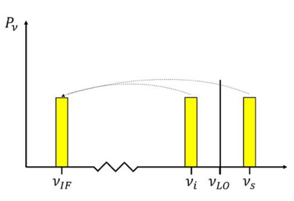
Fig. 2.29 Illustration of the down-conversion process. The measured radio signal is mixed with a local oscillator of frequency  leading to two frequency sidebands leading to two frequency sidebands  and and  . These two sidebands can than be down-converted to an intermediate frequency band at . These two sidebands can than be down-converted to an intermediate frequency band at  , representing the difference between the two sideband frequencies and , respectively. , representing the difference between the two sideband frequencies and , respectively. |
The LO produces a signal at a well-defined and tunable frequency  , close to the observing frequency
  . To mix these two input signals, a semi-conductor diode with a non-linear current-voltage characteristic is used. The current-voltage relation of this diode can be written in terms of a Taylor expansion as
, close to the observing frequency . To mix these two input signals, a semi-conductor diode with a non-linear current-voltage characteristic is used. The current-voltage relation of this diode can be written in terms of a Taylor expansion as = I(U_0) + \frac{\text{d}I}{\text{d}U} \cdot \delta U + \frac{1}{2} \cdot \frac{\text{d}^2 I}{\text{d} U^2} \cdot (\delta U)^2 + \text{...} = K_0 + K_1 \cdot \delta U + K_2 \cdot (\delta U)^2 + \text{...}")
for small variations  around the constant input bias
  of the mixer
 ") , where:
, where:
around the constant input bias of the mixer , where: + B \cdot \sin (\omega_\text{S} \cdot t) \text{,}")
with

Inserting this expression for into the Taylor expansion yields
into the Taylor expansion yields![\displaystyle \begin{array}{rl} I = & K_0 + K_1 \cdot \left[A \cdot \sin (\omega_\text{LO} \cdot t) + B \cdot \sin (\omega_\text{S} \cdot t)\right] \\ & + K_2 \cdot \left[\frac{A^2}{2} + \frac{B^2}{2}\right] \\ & - K_2 \cdot \left[\frac{A^2}{2} \cdot \cos (2 \cdot \omega_\text{LO} \cdot t) + \frac{B^2}{2} \cdot \cos (2 \cdot \omega_\text{S} \cdot t)\right] \\ & + K_2 \cdot A \cdot B \cdot \cos \left[(\omega_\text{LO} - \omega_\text{S}) \cdot t\right] \\ & - K_2 \cdot A \cdot B \cdot \cos \left[(\omega_\text{LO} + \omega_\text{S}) \cdot t\right] \text{,} \end{array}](https://wuecampus.uni-wuerzburg.de/moodle/filter/tex/pix.php/592ca3c1f2371daedb504e40c89cc654.gif "\displaystyle \begin{array}{rl} I = & K_0 + K_1 \cdot \left[A \cdot \sin (\omega_\text{LO} \cdot t) + B \cdot \sin (\omega_\text{S} \cdot t)\right] \\ & + K_2 \cdot \left[\frac{A^2}{2} + \frac{B^2}{2}\right] \\ & - K_2 \cdot \left[\frac{A^2}{2} \cdot \cos (2 \cdot \omega_\text{LO} \cdot t) + \frac{B^2}{2} \cdot \cos (2 \cdot \omega_\text{S} \cdot t)\right] \\ & + K_2 \cdot A \cdot B \cdot \cos \left[(\omega_\text{LO} - \omega_\text{S}) \cdot t\right] \\ & - K_2 \cdot A \cdot B \cdot \cos \left[(\omega_\text{LO} + \omega_\text{S}) \cdot t\right] \text{,} \end{array}")
leading to a frequency spectrum containing frequencies of

Since the LO power  of higher harmonics decreases as
  and usually the signal power
  , only three terms of this frequency spectrum are important, namely:
of higher harmonics decreases as and usually the signal power , only three terms of this frequency spectrum are important, namely:the frequency sum

the intermediate frequency (IF)

and the image frequency

which is the "image" of . Combining these terms, one obtains two high frequency (HF) bands that have equidistant separations from which correspond to the IF. For  , these two HF bands correspond to the observing frequency, or signal frequency, , and the image frequency , and are denoted by
. Combining these terms, one obtains two high frequency (HF) bands that have equidistant separations from which correspond to the IF. For , these two HF bands correspond to the observing frequency, or signal frequency, , and the image frequency , and are denoted by
Figure 2.26 illustrates the down-conversion of the two HF bands to the single IF band. The two HF bands and are called lower sideband (LSB) and upper sideband (USB), respectively. If both sidebands are used, the receiver operates in the so-called double-sideband mode. Otherwise, the receiver is said to operate in the single-sideband mode. To make sure that only the two HF bands are produced by the mixing process, an IF filter is used after the mixer to suppress all unwanted products of the mixing process (e.g.  ).
).
and are called lower sideband (LSB) and upper sideband (USB), respectively. If both sidebands are used, the receiver operates in the so-called double-sideband mode. Otherwise, the receiver is said to operate in the single-sideband mode. To make sure that only the two HF bands are produced by the mixing process, an IF filter is used after the mixer to suppress all unwanted products of the mixing process (e.g. ).Advantages
 |
|---|
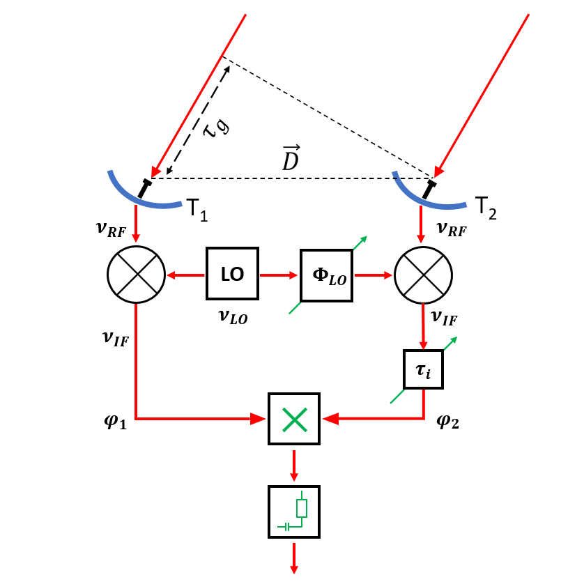
Fig. 2.30 Illustration of the down-conversion process for a two-element interferometer. The measured radio signal at frequency  is mixed with a common local oscillator (LO) signal at frequency . One of the two LO signals is phase-shifted by is mixed with a common local oscillator (LO) signal at frequency . One of the two LO signals is phase-shifted by  . . |
Once the HF bands are down-converted to the lower IF band, further amplification can be performed. Because of the lower frequency, all electronic components after the mixer become more stable and easier to handle. Furthermore, after the heterodyne frequency conversion it is also possible to vary the observing frequency without changing any components following the mixer, which is essential for spectral-line measurements.
without changing any components following the mixer, which is essential for spectral-line measurements.The heterodyne frequency conversion also results in some important advantages in radio interferometry. As already seen before, the correlated power of a two-element interferometer is given by
 \text{,}")
in which  and
and  are the amplitude and phase of the complex visibility function,
  is the baseline between the two antennas in units of the observing wavelength and
  denotes the position of the observed radio source.
and are the amplitude and phase of the complex visibility function, is the baseline between the two antennas in units of the observing wavelength and denotes the position of the observed radio source.Figure 2.27 illustrates such an interferometer with some modifications concerning the heterodyne frequency conversion. First, an artificial time lag  is introduced in one of the two branches of the receiver systems before the correlator. Second, a common LO signal is introduced into both mixers, with a phase shifter fed into one of the branches. Therefore, the resulting signal frequency
  is given by
is introduced in one of the two branches of the receiver systems before the correlator. Second, a common LO signal is introduced into both mixers, with a phase shifter fed into one of the branches. Therefore, the resulting signal frequency is given by
Observing in the single-sideband mode, the USB ") and LSB
and LSB ") phases
phases  and
and  of the two signals are given by
and LSB phases and of the two signals are given by \cdot \tau_\text{g} \text{,}")

in which  is the geometric time delay and is the phase difference between the LO signals at the input of the mixers. The correlated power of such an interferometer can then be determined by changing the phase
  by
by  , leading to
is the geometric time delay and is the phase difference between the LO signals at the input of the mixers. The correlated power of such an interferometer can then be determined by changing the phase by , leading to![\displaystyle P = A_0 \cdot \Delta \nu \cdot |V| \cdot \cos [2 \pi (\nu_\text{LO} \cdot \tau_\text{g} \pm \nu_\text{IF} \cdot \Delta \tau) - \varphi_\text{V} - \varphi_\text{LO}] \text{,}](https://wuecampus.uni-wuerzburg.de/moodle/filter/tex/pix.php/b0bdf3019af0affc0b3b21ed44cbc7bc.gif "\displaystyle P = A_0 \cdot \Delta \nu \cdot |V| \cdot \cos [2 \pi (\nu_\text{LO} \cdot \tau_\text{g} \pm \nu_\text{IF} \cdot \Delta \tau) - \varphi_\text{V} - \varphi_\text{LO}] \text{,}")
in which  .
.
.Therefore, using heterodyne frequency conversion in radio interferometry leads to the possibility that the geometric delay can be compensated by introducing an intrinsic time lag and that any phase variations due to the varying can be compensated by controlling .
can be compensated by introducing an intrinsic time lag and that any phase variations due to the varying can be compensated by controlling . Fringe rotation and complex correlators
By varying , the fringe frequency at which the interference pattern changes for each telescope pair due to the varying hour angle can be reduced. This is called fringe rotation. Looking at the time derivative of , given by
, the fringe frequency at which the interference pattern changes for each telescope pair due to the varying hour angle can be reduced. This is called fringe rotation. Looking at the time derivative of , given by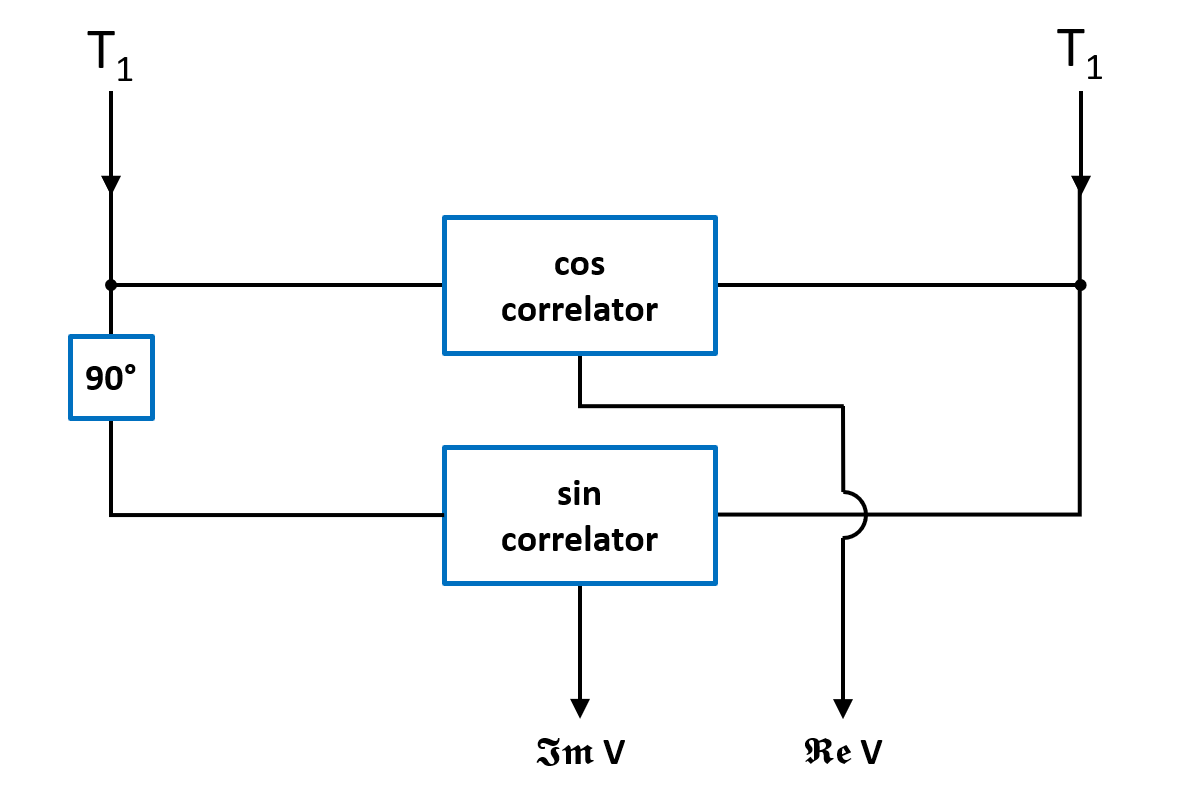 |
|---|
FIg. 2.31 Sketch of a complex correlator. The correlation of the two original signals with a cosine correlator yields the real part of the visibility. The correlation of the two signals, with one of them shifted by  , leads to the imaginary part of the visibility using a sine correlator. , leads to the imaginary part of the visibility using a sine correlator. |
 = 2\pi\cdot\nu_\text{LO}\cdot \frac{\text{d}\tau_\text{g}}{\text{d}t}- \frac{\text{d}\varphi_\text{LO}}{\text{d}t}\,\text{,}")
one can see that it is even possible to stop the fringes by varying at a speed that is identical to the so-called natural fringe frequency, given by the term
at a speed that is identical to the so-called natural fringe frequency, given by the term
This is then called fringe stopping. After rotating or stopping the fringes, it is also much easier to measure the amplitude and phase of the complex visibility by using a so-called complex correlator (see Fig. 2.28). Here, two correlations are performed: one with the two original signals, leading to a co-sinusoidal output signal that represents the real part of the visibility  , and one that has a -phase shift in one of its branches prior to the correlation, leading to a sinusoidal output signal that corresponds to the imaginary part of the visibility
  . With these output signals, the amplitude and phase of the visibility can be calculated by
, and one that has a -phase shift in one of its branches prior to the correlation, leading to a sinusoidal output signal that corresponds to the imaginary part of the visibility . With these output signals, the amplitude and phase of the visibility can be calculated by^2 + (\Im V)^2}")
and
\,\text{.}")