Lecture - Fundamental Concepts
| Sitio: | WueCampus |
| Curso: | vhb : Radio-Astronomical Interferometry (DEMO) |
| Libro: | Lecture - Fundamental Concepts |
| Imprimido por: | Gast |
| Día: | miércoles, 22 de julio de 2026, 06:26 |
1. Fourier optics
Learning Objectives:
- Basic concepts applied to telescopes
- Fourier and convolution mathematics
- Application of telescopes as spatial filters
2. Interferometry
Learning Objectives:
- Interferometry basics and concepts
- Application in radio astronomy
- Introduction to important values like visibility function and bandwidth
- Influences of the instrument set up to the measured values
- Orientation of pointing in the scope of coordinates
3. Aperture Synthesis by Radio Interferometric Arrays
Learning Objectives:
- Establishing a familiarity with the
") space
space - Interferometer arrangements with their strengths and draw backs
- Interferometer properties based on their field of application
4. Receiver Response
Learning Objectives:
- Process and advantages of heterodyne frequency conversion
- Sensitivity of a radio-interferometrical array
- Effects of sampling, weighting and gridding
- Effect of finite bandwidth, bandwidth smearing
- Calibration of radio-interferometrical observations
4.1. Heterodyne frequency conversion
 to work in the quadratic regime. The power
  of the weak radio-astronomical signals entering the receiver is given by
 is the Boltzmann constant and
  is the system temperature containing the receiver noise temperature and the antenna temperature. The antenna temperature is composed of the desired astronomical signal, a contribution from the earth's atmosphere, and possibly radiation from the ground. Due to that always present background the best case for the systemtemperature is
  . Therefore, using a typical bandwidth of
  , the input power
  , meaning that the signal must be amplified by a factor of
  . However, amplification with such high factors is problematic, since the amplifying system becomes unstable due to feedback. A small amount of the power passing through the individual electronic components leaks out and reaches previous receiver elements, where it is again amplified. To circumvent this problem, the frequency of the signal
  is down-converted to the lower intermediate frequency (IF) by mixing the signal with that of a local oscillator (LO), which decouples the signal path after the first amplification. This process is called heterodyne amplification or heterodyne frequency conversion.
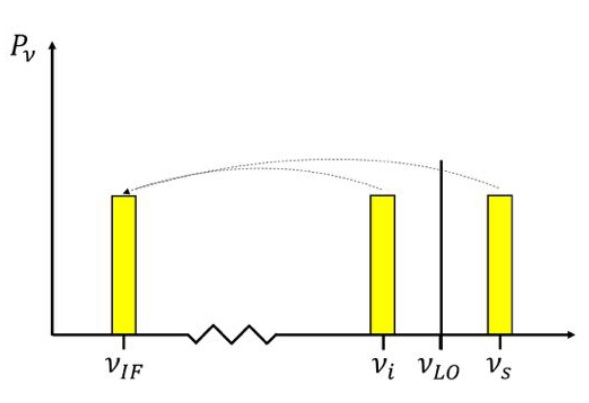 |
|---|
Fig. 2.29 Illustration of the down-conversion process. The measured radio signal is mixed with a local oscillator of frequency  leading to two frequency sidebands leading to two frequency sidebands  and and  . These two sidebands can than be down-converted to an intermediate frequency band at . These two sidebands can than be down-converted to an intermediate frequency band at  , representing the difference between the two sideband frequencies and , respectively. , representing the difference between the two sideband frequencies and , respectively. |
 , close to the observing frequency
  . To mix these two input signals, a semi-conductor diode with a non-linear current-voltage characteristic is used. The current-voltage relation of this diode can be written in terms of a Taylor expansion as
 = I(U_0) + \frac{\text{d}I}{\text{d}U} \cdot \delta U + \frac{1}{2} \cdot \frac{\text{d}^2 I}{\text{d} U^2} \cdot (\delta U)^2 + \text{...} = K_0 + K_1 \cdot \delta U + K_2 \cdot (\delta U)^2 + \text{...}")
 around the constant input bias
  of the mixer
 ") , where:
, where: + B \cdot \sin (\omega_\text{S} \cdot t) \text{,}")
 into the Taylor expansion yields
![\displaystyle \begin{array}{rl} I = & K_0 + K_1 \cdot \left[A \cdot \sin (\omega_\text{LO} \cdot t) + B \cdot \sin (\omega_\text{S} \cdot t)\right] \\ & + K_2 \cdot \left[\frac{A^2}{2} + \frac{B^2}{2}\right] \\ & - K_2 \cdot \left[\frac{A^2}{2} \cdot \cos (2 \cdot \omega_\text{LO} \cdot t) + \frac{B^2}{2} \cdot \cos (2 \cdot \omega_\text{S} \cdot t)\right] \\ & + K_2 \cdot A \cdot B \cdot \cos \left[(\omega_\text{LO} - \omega_\text{S}) \cdot t\right] \\ & - K_2 \cdot A \cdot B \cdot \cos \left[(\omega_\text{LO} + \omega_\text{S}) \cdot t\right] \text{,} \end{array}](https://wuecampus.uni-wuerzburg.de/moodle/filter/tex/pix.php/592ca3c1f2371daedb504e40c89cc654.gif "\displaystyle \begin{array}{rl} I = & K_0 + K_1 \cdot \left[A \cdot \sin (\omega_\text{LO} \cdot t) + B \cdot \sin (\omega_\text{S} \cdot t)\right] \\ & + K_2 \cdot \left[\frac{A^2}{2} + \frac{B^2}{2}\right] \\ & - K_2 \cdot \left[\frac{A^2}{2} \cdot \cos (2 \cdot \omega_\text{LO} \cdot t) + \frac{B^2}{2} \cdot \cos (2 \cdot \omega_\text{S} \cdot t)\right] \\ & + K_2 \cdot A \cdot B \cdot \cos \left[(\omega_\text{LO} - \omega_\text{S}) \cdot t\right] \\ & - K_2 \cdot A \cdot B \cdot \cos \left[(\omega_\text{LO} + \omega_\text{S}) \cdot t\right] \text{,} \end{array}")

 of higher harmonics decreases as
  and usually the signal power
  , only three terms of this frequency spectrum are important, namely:

 . Combining these terms, one obtains two high frequency (HF) bands that have equidistant separations from which correspond to the IF. For
  , these two HF bands correspond to the observing frequency, or signal frequency, , and the image frequency , and are denoted by
 and are called lower sideband (LSB) and upper sideband (USB), respectively. If both sidebands are used, the receiver operates in the so-called double-sideband mode. Otherwise, the receiver is said to operate in the single-sideband mode. To make sure that only the two HF bands are produced by the mixing process, an IF filter is used after the mixer to suppress all unwanted products of the mixing process (e.g.
  ).
). |
|---|
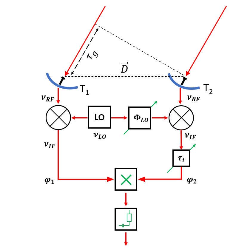
Fig. 2.30 Illustration of the down-conversion process for a two-element interferometer. The measured radio signal at frequency  is mixed with a common local oscillator (LO) signal at frequency . One of the two LO signals is phase-shifted by is mixed with a common local oscillator (LO) signal at frequency . One of the two LO signals is phase-shifted by  . . |
without changing any components following the mixer, which is essential for spectral-line measurements. \text{,}")
 and
and  are the amplitude and phase of the complex visibility function,
  is the baseline between the two antennas in units of the observing wavelength and
  denotes the position of the observed radio source.
 is introduced in one of the two branches of the receiver systems before the correlator. Second, a common LO signal is introduced into both mixers, with a phase shifter fed into one of the branches. Therefore, the resulting signal frequency
  is given by
") and LSB
and LSB ") phases
phases  and
and  of the two signals are given by
 \cdot \tau_\text{g} \text{,}")

 is the geometric time delay and is the phase difference between the LO signals at the input of the mixers. The correlated power of such an interferometer can then be determined by changing the phase
  by
by  , leading to
![\displaystyle P = A_0 \cdot \Delta \nu \cdot |V| \cdot \cos [2 \pi (\nu_\text{LO} \cdot \tau_\text{g} \pm \nu_\text{IF} \cdot \Delta \tau) - \varphi_\text{V} - \varphi_\text{LO}] \text{,}](https://wuecampus.uni-wuerzburg.de/moodle/filter/tex/pix.php/b0bdf3019af0affc0b3b21ed44cbc7bc.gif "\displaystyle P = A_0 \cdot \Delta \nu \cdot |V| \cdot \cos [2 \pi (\nu_\text{LO} \cdot \tau_\text{g} \pm \nu_\text{IF} \cdot \Delta \tau) - \varphi_\text{V} - \varphi_\text{LO}] \text{,}")
 . can be compensated by introducing an intrinsic time lag and that any phase variations due to the varying can be compensated by controlling . , the fringe frequency at which the interference pattern changes for each telescope pair due to the varying hour angle can be reduced. This is called fringe rotation. Looking at the time derivative of , given by
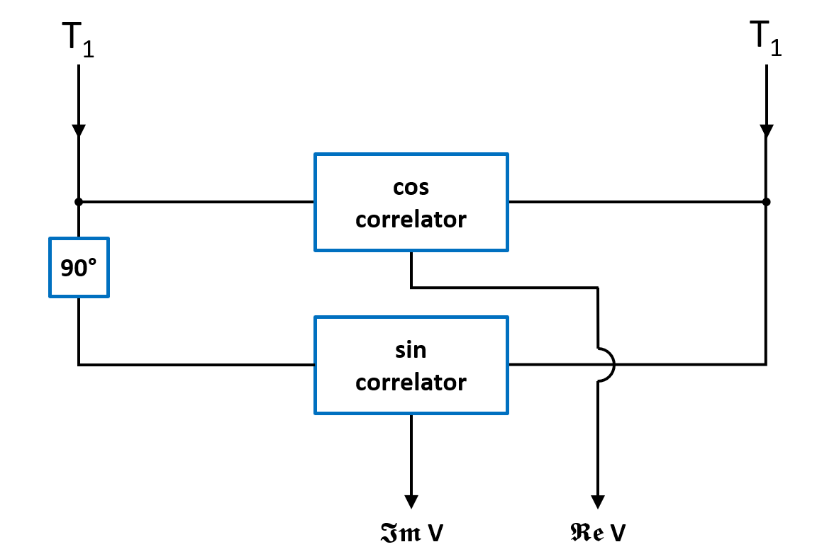 |
|---|
FIg. 2.31 Sketch of a complex correlator. The correlation of the two original signals with a cosine correlator yields the real part of the visibility. The correlation of the two signals, with one of them shifted by  , leads to the imaginary part of the visibility using a sine correlator. , leads to the imaginary part of the visibility using a sine correlator. |
 = 2\pi\cdot\nu_\text{LO}\cdot \frac{\text{d}\tau_\text{g}}{\text{d}t}- \frac{\text{d}\varphi_\text{LO}}{\text{d}t}\,\text{,}") at a speed that is identical to the so-called natural fringe frequency, given by the term
at a speed that is identical to the so-called natural fringe frequency, given by the term
 , and one that has a -phase shift in one of its branches prior to the correlation, leading to a sinusoidal output signal that corresponds to the imaginary part of the visibility
  . With these output signals, the amplitude and phase of the visibility can be calculated by
^2 + (\Im V)^2}")
\,\text{.}")
4.2. Interferometer sensitivity
In order to estimate whether a source can be detected by a radio telescope or array, the so-called signal-to-noise ratio (SNR) has to be calculated. For a single telescope the signal is given by the measured antenna temperature  and the noise is given by the radiometer equation
in which  is a dimensionless constant depending on the receiver system used, is the system temperature,
  is the bandwidth of the receiver equipment and
  is the integration time.
In radio interferometry, the signal is given by the brightness distribution ") of a source that must be calculated by the Fourier integral of the measured visibility
of a source that must be calculated by the Fourier integral of the measured visibility ") :
: = \int_{-\infty}^{\infty} \int_{-\infty}^{\infty} V(u,v) \cdot \text{e}^{\text{i}\cdot 2\pi \cdot (u \cdot \xi + v \cdot \eta)} \text{d}u ~\text{d}v \text{.}")
Therefore, to calculate the SNR in radio interferometry, one has to calculate the uncertainty of the brightness distribution  from the uncertainty of the complex visibility
  . As in every measurement, the measured data need to be sampled, meaning that the visibility is only measured at discrete locations
 ") along the tracks in the -plane. Let:
along the tracks in the -plane. Let:  be the integration time of the individual samples in the -plane,
  be the total integration time and
  be the total number of antennas. Then the total number of measured visibilities
  is given by
in which}{2}")
is the number of antenna pairs or rather the number of individual two-element interferometers. Since this brightness distribution suffers from incomplete -coverage, the resulting image is called a "dirty image", which is also indicated by the superscript "D" of the brightness distribution ") . The visibilities are measured at discrete locations , so the brightness distribution is given by the discrete Fourier transform
. The visibilities are measured at discrete locations , so the brightness distribution is given by the discrete Fourier transform = K \cdot \sum_{\text{l}=0}^{2\cdot n_\text{d}} V(u,v) \cdot S(u,v) \cdot \text{e}^{\text{i}\cdot 2\pi \cdot (u \cdot \xi_\text{m} + v \cdot \eta_\text{m})} \text{,}")
in which  is a normalization constant and
 ") is a sampling function which is given by
is a sampling function which is given by = \sum_{\text{l}=0}^{2\cdot n_\text{d}} \delta^2(u - u_\text{l}, v - v_\text{l}) \text{.}")
This sampling function is only non-zero where the visibility is measured in the -plane.
To suppress sidelobes, the beam shape of the observing array can be controlled by applying appropriate weights to the measured visibilities. Furthermore, if the observing array consists of telescopes that have different collecting areas  , and different receivers with different system temperatures , frequency bandwidths
  and integration times , one can also apply weights to control these differences. The weights can be written as
 = \sum_{\text{l}=0}^{2\cdot n_\text{d}} R_\text{l} \cdot T_\text{l} \cdot D_\text{l} \cdot \delta^2(u - u_\text{l}, v - v_\text{l}) \text{,}")
in which  accounts for different telescope properties,
  is a taper which controls the beam shape and
  weights the density of the measured visibilities (more detailed information on the weights, especially on the -factor, will be given in the next section 2.4.3). With these weights, the brightness distribution can then be written as
 = K \cdot \sum_{\text{l}=0}^{2\cdot n_\text{d}} V(u,v) \cdot S(u,v) \cdot W(u,v) \cdot \text{e}^{\text{i}\cdot 2\pi \cdot (u \cdot \xi_\text{m} + v \cdot \eta_\text{m})} \text{.}")
Because there is no measurement in the center of the -plane, the  terms of the dirty image vanish, leading to
![\displaystyle \begin{array}{rl} B^\text{D}(\xi_\text{m}, \eta_\text{m}) & = K \cdot \sum_{\text{l}=0}^{2\cdot n_\text{d}} V_\text{l} \cdot W_\text{l} \cdot \text{e}^{\text{i}\cdot 2\pi \cdot (u_\text{l} \cdot \xi_\text{m} + v_\text{l} \cdot \eta_\text{m})} \\ & = 2 \cdot K \cdot \sum_{\text{l}=1}^{n_\text{d}} W_\text{l} \cdot [ \Re V_\text{l} \cdot \cos(2\pi \cdot (u_\text{l} \cdot \xi_\text{m} + v_\text{l} \cdot \eta_\text{m})) - \Im V_\text{l} \cdot \sin(2\pi \cdot (u_\text{l} \cdot \xi_\text{m} + v_\text{l} \cdot \eta_\text{m}))] \text{,} \end{array}](https://wuecampus.uni-wuerzburg.de/moodle/filter/tex/pix.php/04c07eca8079ad16147719b4c40cf6be.gif "\displaystyle \begin{array}{rl} B^\text{D}(\xi_\text{m}, \eta_\text{m}) & = K \cdot \sum_{\text{l}=0}^{2\cdot n_\text{d}} V_\text{l} \cdot W_\text{l} \cdot \text{e}^{\text{i}\cdot 2\pi \cdot (u_\text{l} \cdot \xi_\text{m} + v_\text{l} \cdot \eta_\text{m})} \\ & = 2 \cdot K \cdot \sum_{\text{l}=1}^{n_\text{d}} W_\text{l} \cdot [ \Re V_\text{l} \cdot \cos(2\pi \cdot (u_\text{l} \cdot \xi_\text{m} + v_\text{l} \cdot \eta_\text{m})) - \Im V_\text{l} \cdot \sin(2\pi \cdot (u_\text{l} \cdot \xi_\text{m} + v_\text{l} \cdot \eta_\text{m}))] \text{,} \end{array}")
in which \cdot S(u,v) = \Re V_\text{l} + \text{i} \cdot \Im V_\text{l}")
and \text{.}")
Note that the two additional terms ![\Re V_\text{l} \cdot \sin[2\pi \cdot (u_\text{l} \cdot \xi_\text{m} + v_\text{l} \cdot \eta_\text{m})]](https://wuecampus.uni-wuerzburg.de/moodle/filter/tex/pix.php/50a8ee2bb161b4b41f5ab85faa62b859.gif "\Re V_\text{l} \cdot \sin[2\pi \cdot (u_\text{l} \cdot \xi_\text{m} + v_\text{l} \cdot \eta_\text{m})]") and
and ![\Im V_\text{l} \cdot \cos[2\pi \cdot (u_\text{l} \cdot \xi_\text{m} + v_\text{l} \cdot \eta_\text{m})]](https://wuecampus.uni-wuerzburg.de/moodle/filter/tex/pix.php/30bd73fb80f7725027d8515833593296.gif "\Im V_\text{l} \cdot \cos[2\pi \cdot (u_\text{l} \cdot \xi_\text{m} + v_\text{l} \cdot \eta_\text{m})]") vanish under the integral of and can therefore also be neglected for the sum of
vanish under the integral of and can therefore also be neglected for the sum of ") .
.
To calculate the sensitivity in the image plane, a point source at the phase and image center is considered. For such a point source, the visibility is real and constant across the entire -plane and only varies due to random noise. Furthermore, because  , the
, the ![\sin[2\pi \cdot (u_\text{l} \cdot \xi_\text{m} + v_\text{l} \cdot \eta_\text{m})]](https://wuecampus.uni-wuerzburg.de/moodle/filter/tex/pix.php/9b252b33edecca4b4f2300bbdd905d3b.gif "\sin[2\pi \cdot (u_\text{l} \cdot \xi_\text{m} + v_\text{l} \cdot \eta_\text{m})]") -term vanishes and
-term vanishes and ![\cos[2\pi \cdot (u_\text{l} \cdot \xi_\text{m} + v_\text{l} \cdot \eta_\text{m})] = 1](https://wuecampus.uni-wuerzburg.de/moodle/filter/tex/pix.php/423a918ff62e58d89f2ee83a7f9b4ea6.gif "\cos[2\pi \cdot (u_\text{l} \cdot \xi_\text{m} + v_\text{l} \cdot \eta_\text{m})] = 1") . Therefore, the dirty image of such a point source is given by
. Therefore, the dirty image of such a point source is given by & = 2 \cdot K \cdot \sum_{\text{l}=1}^{n_\text{d}} W_\text{l} \cdot \Re V_\text{l} \\& = 2 \cdot K \cdot \sum_{\text{l}=1}^{n_\text{d}} W_\text{l} \cdot S_\text{l} \\& = 2 \cdot K \cdot S \cdot \sum_{\text{l}=1}^{n_\text{d}} W_\text{l} \text{,} \end{array}")
in which  is the total flux density of the source. Note that here
so that = S \text{.}")
Assuming that the uncertainty of the flux density  , the noise in the dirty image is given by
Furthermore, assuming an observing array that consists of identical telescopes ") and a naturally weighted
and a naturally weighted ") , untapered
, untapered ") image,
image,  simplifies to
Since  , the uncertainty of the flux density
  is given by the rms noise
  of the measured visibilities which is, based on the radiometer equation, given by
in which is the Boltzmann constant and
is the quantization efficiency accounting for the quantization noise due to the conversion of analogue signals to digital signals.
Inserting  into , the sensitivity for the synthesized image is finally given by
}{2} \cdot \Delta \nu_\text{IF} \cdot \tau_0}} \text{.}")
4.3. Sampling, weighting, gridding
Sampling
As previously mentioned, the visibilities are only measured at discrete locations ") . Therefore, the measured visibilities are given by the multiplication of the true visibility function and a sampling function
. Therefore, the measured visibilities are given by the multiplication of the true visibility function and a sampling function  . Hence, the dirty image
  is then given by the convolution of their Fourier transforms:
![\displaystyle B^\text{D} = \mathcal{FT}[V^\text{S}] = \mathcal{FT}[V \cdot S] = \mathcal{FT}[V] \star \star \mathcal{FT}[S] \text{,}](https://wuecampus.uni-wuerzburg.de/moodle/filter/tex/pix.php/ae19d1b8e17a3ebbdd115e1eeff5e233.gif "\displaystyle B^\text{D} = \mathcal{FT}[V^\text{S}] = \mathcal{FT}[V \cdot S] = \mathcal{FT}[V] \star \star \mathcal{FT}[S] \text{,}")
in which ![\mathcal{FT}[x]](https://wuecampus.uni-wuerzburg.de/moodle/filter/tex/pix.php/290d52c31264c1e54193648e665e8ad5.gif "\mathcal{FT}[x]") denotes the Fourier transform of
denotes the Fourier transform of  and the double-star
  indicates a two-dimensional convolution.
Weighting
Furthermore, as also previously mentioned, the visibilities can be weighted by multiplying a weighting function  to the visibilities
  :
:

This weighting function consists of three individual factors:
- accounts for different telescope properties within an array (e.g. different , , and ),
- is a taper that controls the beam shape,
- weights the density of the measured visibilities.
The -factor affects the angular resolution and sensitivity of the array. On the one hand side, the highest angular resolution can be achieved by weighting the visibilities as if they had been measured uniformly over the entire -plane. Therefore, this weighting scheme is called uniform weighting. Since the density of the measured visibilities is higher at the center of the -plane, the visibilities in the outer part are over-weighted leading to the highest angular resolution. On the other hand, the highest sensitivity is achieved if all measured visibilities are weighted by identical weights. This weighting scheme is called natural weighting. The main properties of both schemes are summarized in the following:
- natural weighting:

- broader synthesized beam
- highest sensitivity
- uniform weighting:
}") , in which
, in which ") is the number of visibilities occurring within an area of constant size around the weighted visibility
is the number of visibilities occurring within an area of constant size around the weighted visibility- highest resolution
- lowest sensitivity
With this weighting function , the dirty image is given by
![\displaystyle B^\text{D} = \mathcal{FT}[V^\text{W}] = \mathcal{FT}[W \cdot V^\text{S}] = \mathcal{FT}[W] \star \star \mathcal{FT}[V^\text{S}] = \mathcal{FT}[W] \star \star (\mathcal{FT}[V] \star \star \mathcal{FT}[S]) \text{.}](https://wuecampus.uni-wuerzburg.de/moodle/filter/tex/pix.php/2eca0fb08d98b8eadba80a378194ca7b.gif "\displaystyle B^\text{D} = \mathcal{FT}[V^\text{W}] = \mathcal{FT}[W \cdot V^\text{S}] = \mathcal{FT}[W] \star \star \mathcal{FT}[V^\text{S}] = \mathcal{FT}[W] \star \star (\mathcal{FT}[V] \star \star \mathcal{FT}[S]) \text{.}")
Gridding
To use the time advantage of the fast Fourier transform (FFT) algorithm, the visibilities must be interpolated onto a regular grid of size ") , resulting in an image of size
, resulting in an image of size  . This interpolation, also called gridding, is done at first by convolving the weighted discrete visibility
  with an appropriate function to obtain a continuous visibility distribution. This continuous visibility distribution is then resampled at points of the regular grid with spacings
  and
and  by multiplying a two-dimensional Shah-function
  , given by
 |
|---|
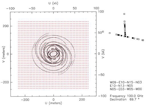
Fig. 2.32 Illustration of the gridding process. The real -tracks measured by the IRAM interferometer at Plateau de Bure in France (black dots) have to be interpolated onto a regular grid of  pixels (red dots). Taken from: U. Klein pixels (red dots). Taken from: U. Klein |
 = \sum_{\text{j} = -\infty}^{\infty} \sum_{\text{k} = -\infty}^{\infty} \delta^2\left(j-\frac{u}{\Delta u}, k-\frac{v}{\Delta v}\right) \text{.}")
After these modifications, the visibility  is given by
 ![\displaystyle V^\text{G} = G \cdot (C \star \star V^\text{W}) = G \cdot [C \star \star (W \cdot V^\text{S})] = G \cdot [C \star \star (W \cdot V \cdot S)]](https://wuecampus.uni-wuerzburg.de/moodle/filter/tex/pix.php/24e98dae931507ec8c75522931b13c87.gif "\displaystyle V^\text{G} = G \cdot (C \star \star V^\text{W}) = G \cdot [C \star \star (W \cdot V^\text{S})] = G \cdot [C \star \star (W \cdot V \cdot S)]")
and the dirty image  reads
reads![\displaystyle \tilde{B^\text{D}} = \mathcal{FT}[G] \star \star (\mathcal{FT}[C] \cdot \mathcal{FT}[V^\text{W}]) = \mathcal{FT}[G] \star \star \{ \mathcal{FT}[C] \cdot [\mathcal{FT}[W] \star \star (\mathcal{FT}[V] \star \star \mathcal{FT}[S])]\} \text{.}](https://wuecampus.uni-wuerzburg.de/moodle/filter/tex/pix.php/1b44c8e537f9f7143cf62d73d416bec3.gif "\displaystyle \tilde{B^\text{D}} = \mathcal{FT}[G] \star \star (\mathcal{FT}[C] \cdot \mathcal{FT}[V^\text{W}]) = \mathcal{FT}[G] \star \star \{ \mathcal{FT}[C] \cdot [\mathcal{FT}[W] \star \star (\mathcal{FT}[V] \star \star \mathcal{FT}[S])]\} \text{.}")
This gridding process is illustrated in the Fig. 2.29, in which real -tracks measured by the IRAM interferometer at Plateau de Bure in France are shown as black dotted ellipses. Furthermore, a regular grid, onto which the visibilities have been interpolated, is shown as red dots.
Since the sampling intervals and in the -plane are inversely proportional to the sampling intervals  and
and  in the image plane (
  and
and  for a grid of size
  ), the maximum map size in one domain is given by the minimum sampling interval in the other. Therefore, it is important to choose appropriate sampling intervals and . If and are chosen to be too large for example, this will result in artefacts in the image plane produced by reflections of structures from the map edges, which is called aliasing.
The most effective way to deal with this aliasing is to use a convolution function for which the Fourier transform in the image plane ![\mathcal{FT}[C]](https://wuecampus.uni-wuerzburg.de/moodle/filter/tex/pix.php/7265b9d7b7857f89d7fdad5bc301eb5a.gif "\mathcal{FT}[C]") decreases rapidly at the image edges and is nearly constant over the image. Therefore, the simplest choice for the convolution function is a rectangular function, but with this choice the aliasing would be strongest. A better choice would be a sinc function, however a Gaussian-sinc function (product of a Gaussian and a sinc function) leads to the best suppression of aliasing.
decreases rapidly at the image edges and is nearly constant over the image. Therefore, the simplest choice for the convolution function is a rectangular function, but with this choice the aliasing would be strongest. A better choice would be a sinc function, however a Gaussian-sinc function (product of a Gaussian and a sinc function) leads to the best suppression of aliasing.
Finally, the gridding modifications must be corrected after the Fourier transform by dividing the dirty image ") by the inverse Fourier transform of the gridding convolution function
by the inverse Fourier transform of the gridding convolution function ") . Therefore, the so-called grid-corrected image
. Therefore, the so-called grid-corrected image ") is given by
is given by} \text{.}](https://wuecampus.uni-wuerzburg.de/moodle/filter/tex/pix.php/38a39a2ff58598a9e9090adcf122a3df.gif "\displaystyle \tilde{B^\text{D}_\text{C}}(\xi_\text{m},\eta_\text{m}) = \frac{\tilde{B^\text{D}}(\xi_\text{m},\eta_\text{m})}{\mathcal{FT}[C](u,v)} \text{.}")
4.4. Bandwidth smearing
As already seen in Chapt. 2 Sect. 4.2, the sensitivity of radio-interferometrical measurements depends on the effective area of the telescopes and the bandwidth . The larger , the higher the sensitivity. However, using a large bandwidth is problematic, since the Fourier relation between brightness distribution and visibility is only valid for monochromatic signals. Therefore, the effects of the finite bandwidth on the images obtained from radio-interferometrical observations, especially the inevitable effect called bandwidth smearing or chromatic aberration, will be investigated in this section, following the textbook of Taylor et al. (1999).
For a single observing frequency  the brightness distribution is given by
 = \int_{-\infty}^{\infty}\int_{-\infty}^{\infty}\tilde{V}(u_0,v_0)\cdot \text{e}^{2\pi\text{i}\cdot(u_0\xi+v_0\eta)}\text{d}u_0\text{d}v_0\text{,}")
in which the "~" indicates the influence of a bandpass. The frequency-independent coordinates  and
and  are given by

where  and
and  are the actual spatial coordinates of the visibility at the frequency
  .
.
Therefore, using the generalized similarity theorem for Fourier transformations in  dimensions, which reads
![\displaystyle \mathcal{FT}^n[f(\alpha\vec{x})] = \frac{1}{|\alpha|^n}\cdot F\left(\frac{\vec{s}}{\alpha}\right)\text{,}](https://wuecampus.uni-wuerzburg.de/moodle/filter/tex/pix.php/2a07d6755df3f8f9491bf87c0848d26b.gif "\displaystyle \mathcal{FT}^n[f(\alpha\vec{x})] = \frac{1}{|\alpha|^n}\cdot F\left(\frac{\vec{s}}{\alpha}\right)\text{,}")
the two-dimensional Fourier relation between visibility and brightness distribution is given by
=B\left(\xi_0\frac{\nu_0}{\nu},\eta_0\frac{\nu_0}{\nu}\right)\Leftrightarrow\left(\frac{\nu}{\nu_0}\right)^2\cdot V\left(u_0\frac{\nu}{\nu_0},v_0\frac{\nu}{\nu_0}\right)=\left(\frac{\nu}{\nu_0}\right)^2\cdot V(u,v)\text{.}")
Furthermore, since the smeared visibility ") is obtained by rescaling and weighting the true visibility
is obtained by rescaling and weighting the true visibility ") by a normalized bandpass function
by a normalized bandpass function ") , where
, where  , and then integrating over the frequency band, another important effect must be taken into account. There will be a delay error of

for signals arriving from a direction ") at frequency . Therefore, the phase is shifted by
at frequency . Therefore, the phase is shifted by
\Delta\tau=2\pi\nu'\frac{u_0\xi+v_0\eta}{\nu_0}")
and the smeared visibility is given by
=\int_{-\infty}^{\infty}V\left(u_0\frac{\nu}{\nu_0},v_0\frac{\nu}{\nu_0}\right)\left(\frac{\nu}{\nu_0}\right)^2G_\text{n}(\nu')\text{e}^{2\pi\text{i}\frac{\nu'}{\nu_0}(u_0\xi+v_0\eta)}\text{d}\nu'\text{.}")
For simplicity, a point source with unit amplitude located at ") is assumed without restricting generality. Then, the true visibility is given by
is assumed without restricting generality. Then, the true visibility is given by
=\text{e}^{-2\pi\text{i}u\xi_0}")
and the smeared visibility reads
=\int_{-\infty}^{\infty}\text{e}^{-2\pi\text{i}u_0\frac{\nu}{\nu_0}\xi_0}\left(\frac{\nu}{\nu_0}\right)^2G_\text{n}(\nu')\text{e}^{2\pi\text{i}\frac{\nu'}{\nu_0}(u_0\xi+v_0\eta)}\text{d}\nu'\text{.}")
Furthermore, assuming that the bandwidth is sufficiently small, so that ^2\approx1") (in practice,
(in practice, ^2\lesssim0.998") ), the bandwidth-smeared brightness distribution is given by
), the bandwidth-smeared brightness distribution is given by
![\displaystyle \begin{array}{rl} \tilde{B}(\xi,\eta) & =\int_{-\infty}^{\infty}\left[\int_{-\infty}^{\infty}{e}^{-2\pi\text{i}u_0\frac{\nu}{\nu_0}\xi_0}G_\text{n}(\nu')\text{e}^{2\pi\text{i}u_0\frac{\nu'}{\nu_0}\xi}\text{d}\nu'\right]\text{e}^{2\pi\text{i}u_0\xi}\text{d}u_0\delta(\eta) \\
& =\int_{-\infty}^{\infty}\left[\int_{-\infty}^{\infty}{e}^{-2\pi\text{i}u_0\left(1+\frac{\nu'}{\nu_0}\right)\xi_0}G_\text{n}(\nu')\text{e}^{2\pi\text{i}u_0\frac{\nu'}{\nu_0}\xi}\text{d}\nu'\right]\text{e}^{2\pi\text{i}u_0\xi}\text{d}u_0\delta(\eta) \\
& =\int_{-\infty}^{\infty}\text{e}^{2\pi\text{i}u_0(\xi-\xi_0)}\left[\int_{-\infty}^{\infty}G_\text{n}(\nu')\text{e}^{2\pi\text{i}u_0\frac{\nu'}{\nu_0}(\xi-\xi_0)}\text{d}\nu'\right]\text{d}u_0\delta(\eta)\text{,} \end{array}](https://wuecampus.uni-wuerzburg.de/moodle/filter/tex/pix.php/fad18f927e16c8b02e3b961d3822a48e.gif "\displaystyle \begin{array}{rl} \tilde{B}(\xi,\eta) & =\int_{-\infty}^{\infty}\left[\int_{-\infty}^{\infty}{e}^{-2\pi\text{i}u_0\frac{\nu}{\nu_0}\xi_0}G_\text{n}(\nu')\text{e}^{2\pi\text{i}u_0\frac{\nu'}{\nu_0}\xi}\text{d}\nu'\right]\text{e}^{2\pi\text{i}u_0\xi}\text{d}u_0\delta(\eta) \\
& =\int_{-\infty}^{\infty}\left[\int_{-\infty}^{\infty}{e}^{-2\pi\text{i}u_0\left(1+\frac{\nu'}{\nu_0}\right)\xi_0}G_\text{n}(\nu')\text{e}^{2\pi\text{i}u_0\frac{\nu'}{\nu_0}\xi}\text{d}\nu'\right]\text{e}^{2\pi\text{i}u_0\xi}\text{d}u_0\delta(\eta) \\
& =\int_{-\infty}^{\infty}\text{e}^{2\pi\text{i}u_0(\xi-\xi_0)}\left[\int_{-\infty}^{\infty}G_\text{n}(\nu')\text{e}^{2\pi\text{i}u_0\frac{\nu'}{\nu_0}(\xi-\xi_0)}\text{d}\nu'\right]\text{d}u_0\delta(\eta)\text{,} \end{array}")
using  . Here, one can see that the term in squared brackets is the Fourier transform of the normalized bandpass function over
  , to an argument
 ") that represents a delay corresponding to the positional offset
that represents a delay corresponding to the positional offset  . Therefore, it is helpful to define a delay function
 ") , given by
, given by
 = \int_{-\infty}^{\infty} G_\text{n}(\nu')\text{e}^{2\pi\text{i}\tau\nu'}\text{d}\nu'\text{.}")
Using this delay function, the bandwidth-smeared brightness distribution then reads
=\int_{-\infty}^{\infty}\text{e}^{2\pi\text{i}u_0(\xi-\xi_0)}d(\tau)\text{d}u_0\delta(\eta)\text{.}")
Therefore, the bandwidth-smeared brightness distribution is the Fourier transform over of the product of the true visibility with the delay function. Using the convolution theorem, the brightness distribution is given by
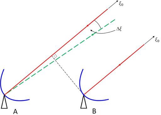 |
|---|
Fig. 2.33 Illustration of the effect of bandwidth smearing. Two signals that arrive from slightly different directions,  and and  , with slightly different frequencies can positively interfere, if their delay difference matches. , with slightly different frequencies can positively interfere, if their delay difference matches. |
=\int_{-\infty}^{\infty}\text{e}^{2\pi\text{i}u_0(\xi-\xi_0)}\text{d} u_0\delta(\eta) \star \int_{-\infty}^{\infty}d(\tau)\text{e}^{2\pi\text{i}u_0 \xi}\text{d} u_0\text{,}")
which is the convolution of the true image with a position-dependent bandwidth distortion function ") , which is the Fourier transform of the delay function
, which is the Fourier transform of the delay function
over . Since this distortion function varies with the radial distance from the phase center and is always oriented along the radius to the phase center, the final image of an extended source can be interpreted as a radially-dependent convolution.
The effect of finite bandwidth is illustrated in Fig. 2.30. Here it is assumed that the observed emission of a source at position positively interferes exactly at frequency . A signal from a neighboring position shifted by  with respect to measured by one telescope at a frequency deviating from by an amount of
  , for example, can then also produce maximum interference with a signal from measured by the other telescope at frequency , if the delay difference matches. Therefore, a source observed with finite bandwidth can also produce structures away from its nominal position.
This finite bandwidth effect cannot be removed, because it is described by a mathematical functional. However, there are two methods to minimize the effects of bandwidth smearing. The first method is to limit the field size by dividing the observed area into subfields and produce separate images for all such subfields. To cover the complete area, the images of the subfields can then be fitted together. This technique is called mosaicing. The second method is to split the full frequency band into narrower sections, which will be summed up after imaging each individual data set. This method is called bandwidth synthesis.
4.5. Calibration
The true visibility of a target source ") observed by two telescopes
observed by two telescopes  and
and  of an array is related to the observed visibility
 ") by
by
=G_\text{ij}(t)\cdot V_\text{ij}^\text{target}(u,v)\text{,}")
in which ") is the time-variable and complex gain factor of the correlation product of the two telescopes and . This gain factor includes variations caused by different effects, e.g., weather effects, effects of the atmospheric paths to the telescopes, and instrumental effects. Therefore, to determine the true visibility, the gain factor has to be calculated. This can be done via frequent observations of calibrator sources with known flux densities
is the time-variable and complex gain factor of the correlation product of the two telescopes and . This gain factor includes variations caused by different effects, e.g., weather effects, effects of the atmospheric paths to the telescopes, and instrumental effects. Therefore, to determine the true visibility, the gain factor has to be calculated. This can be done via frequent observations of calibrator sources with known flux densities  and accurately known positions. Furthermore, these sources have to be point sources, meaning that their angular size
  is
is

Then, the complex gain of each interferometer can be determined by
=G_\text{ij}(t)\cdot S_\text{cal}\text{,}")
in which ") is the observed visibility of a calibrator source. This complex gain factor can then be used to calibrate the observed visibility of the target source. The true visibility of a target source is then given by
is the observed visibility of a calibrator source. This complex gain factor can then be used to calibrate the observed visibility of the target source. The true visibility of a target source is then given by
=\frac{V_\text{ij}^\text{obs}(u,v)}{G_\text{ij}(t)}=V_\text{ij}^\text{obs}(u,v)\cdot\frac{S_\text{cal}}{V_\text{ij}^\text{cal}(u,v)}\text{.}")
Note that the gains  can also be expressed by the voltage gain factors
  and
and  of the individual i-th and j-th antennas by

This reduces the amount of calibration data, since there are many more correlated antenna pairs than antennas in large arrays. Furthermore, this makes the calibration procedure more flexible, since, for example, a source that is resolved at the longest baselines of an array can be used to compute the gain factors of the individual antennas from measurements made only at shorter baselines, at which the source appears unresolved.
Gibb's phenomenon
 |
|---|
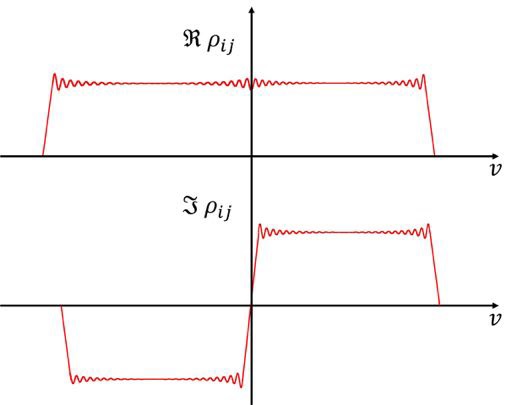
| Fig. 2.34 Real and imaginary part of a frequency power spectrum for an idealized rectangular bandpass. |
In continuum observations the correlation of the signals is usually measured for zero time lags, meaning that the correlation of the measured signal is averaged over the bandwidth, which is defined via a bandpass. In spectral line observations (see Chapt. 3 Sect. 4), measurements at different frequencies across the bandpass are required, which can be implemented by correlating the signals as a function of time lags. After Fourier transforming this correlation output, this yields the so-called cross power spectrum. This cross power spectrum is obtained for  frequency channels (for more detailed information see Chapt. 3 Sect. 4).
To calibrate an interferometer over the bandpass, which represents the filter characteristics of the last IF stage, a continuum point source is used to determine the complex gains of the interferometer, which yields the true cross-correlation spectrum of the observed target source. For calibrator sources with a constant continuum spectrum over the bandpass, the behavior of the complex gains and across the bandpass  are given by the correlated power as a function of frequency for each interferometer of the observing array. The real and imaginary parts of this correlated power, measured for a continuum source with a flat spectrum, are shown in Fig. 2.31 for an idealized rectangular bandpass.
The observed visibility of an unknown target source is given by
![\displaystyle V_\text{ij}^\text{obs}(\nu) = f(\nu)\star\left[g_\text{i}(\nu)\cdot g_\text{j}^\star(\nu)\cdot V(\nu)\right]\,\text{,}](https://wuecampus.uni-wuerzburg.de/moodle/filter/tex/pix.php/7297e6737b5dd7ac508e7e663b3eff7b.gif "\displaystyle V_\text{ij}^\text{obs}(\nu) = f(\nu)\star\left[g_\text{i}(\nu)\cdot g_\text{j}^\star(\nu)\cdot V(\nu)\right]\,\text{,}")
in which ") is the Fourier transform of the truncating function in the frequency domain, which is a sinc function given by
is the Fourier transform of the truncating function in the frequency domain, which is a sinc function given by
 = \frac{\sin(\pi\cdot\nu\cdot K/\Delta\nu)}{\pi\cdot\nu}\,\text{.}")
Here,  is given by a convolution with , since the cross-correlation has only a finite maximum lag of
  . The observed visibility
  of a calibrator source with
  and
and  is then given by
![\displaystyle V_\text{ij}^\text{cal}(\nu)= f(\nu)\star\left[g_\text{i}(\nu)\cdot g_\text{j}^\star(\nu)\right]\,\text{.}](https://wuecampus.uni-wuerzburg.de/moodle/filter/tex/pix.php/ae8aea962d1fb5efc776eeae15172263.gif "\displaystyle V_\text{ij}^\text{cal}(\nu)= f(\nu)\star\left[g_\text{i}(\nu)\cdot g_\text{j}^\star(\nu)\right]\,\text{.}")
Finally, the true visibility  of the observed target source is given by
![\displaystyle V_\text{ij}^\text{true}(\nu) = \frac{V_\text{ij}^\text{obs}(\nu)}{V_\text{ij}^\text{cal}(\nu)} = \frac{f(\nu)\star\left[g_\text{i}(\nu)\cdot g_\text{j}^\star(\nu)\cdot V(\nu)\right]}{f(\nu)\star\left[g_\text{i}(\nu)\cdot g_\text{j}^\star(\nu)\right]}\,\text{,}](https://wuecampus.uni-wuerzburg.de/moodle/filter/tex/pix.php/a8f767a1bf856a6926838936f2d61110.gif "\displaystyle V_\text{ij}^\text{true}(\nu) = \frac{V_\text{ij}^\text{obs}(\nu)}{V_\text{ij}^\text{cal}(\nu)} = \frac{f(\nu)\star\left[g_\text{i}(\nu)\cdot g_\text{j}^\star(\nu)\cdot V(\nu)\right]}{f(\nu)\star\left[g_\text{i}(\nu)\cdot g_\text{j}^\star(\nu)\right]}\,\text{,}")
in which the gains do not cancel out, due to the convolution. Therefore, the original frequency power spectrum, shown in Fig. 2.31, is convolved with the sinc function , due to the finite lag, which will lead to large errors, if the target source has a spectral line near  . This is known as Gibbs' phenomenon.
Since the cross-correlation function has a complex power spectrum, Gibbs' phenomenon has strong influence on the imaginary part of the true visibility, because of the ratio in the equation for , which leads to non-negligible errors, especially for strong line emission near the step at . Since the step in the imaginary part is large, these errors have a strong effect on the phases, producing strong ripples.
5. Image reconstruction
Learning Objectives:
- Image reconstruction using the CLEAN and MEM algorithms
- Image defects
- Image reconstruction using self-calibration
6. Digital Beamforming
Learning Objectives:
- Geometric understanding of an array performing beamforming
- Introduction and mathematical concept of weighting elements
- Mathematical description of one and two dimensional array factors
- Visualization of array factors, beam forming and beam steering