Lecture - Fundamental Concepts
4. Receiver Response
4.5. Calibration
The true visibility of a target source ") observed by two telescopes
observed by two telescopes  and
and  of an array is related to the observed visibility
 ") by
by
=G_\text{ij}(t)\cdot V_\text{ij}^\text{target}(u,v)\text{,}")
in which ") is the time-variable and complex gain factor of the correlation product of the two telescopes and . This gain factor includes variations caused by different effects, e.g., weather effects, effects of the atmospheric paths to the telescopes, and instrumental effects. Therefore, to determine the true visibility, the gain factor has to be calculated. This can be done via frequent observations of calibrator sources with known flux densities
is the time-variable and complex gain factor of the correlation product of the two telescopes and . This gain factor includes variations caused by different effects, e.g., weather effects, effects of the atmospheric paths to the telescopes, and instrumental effects. Therefore, to determine the true visibility, the gain factor has to be calculated. This can be done via frequent observations of calibrator sources with known flux densities  and accurately known positions. Furthermore, these sources have to be point sources, meaning that their angular size
  is
is

Then, the complex gain of each interferometer can be determined by
=G_\text{ij}(t)\cdot S_\text{cal}\text{,}")
in which ") is the observed visibility of a calibrator source. This complex gain factor can then be used to calibrate the observed visibility of the target source. The true visibility of a target source is then given by
is the observed visibility of a calibrator source. This complex gain factor can then be used to calibrate the observed visibility of the target source. The true visibility of a target source is then given by
=\frac{V_\text{ij}^\text{obs}(u,v)}{G_\text{ij}(t)}=V_\text{ij}^\text{obs}(u,v)\cdot\frac{S_\text{cal}}{V_\text{ij}^\text{cal}(u,v)}\text{.}")
Note that the gains  can also be expressed by the voltage gain factors
  and
and  of the individual i-th and j-th antennas by

This reduces the amount of calibration data, since there are many more correlated antenna pairs than antennas in large arrays. Furthermore, this makes the calibration procedure more flexible, since, for example, a source that is resolved at the longest baselines of an array can be used to compute the gain factors of the individual antennas from measurements made only at shorter baselines, at which the source appears unresolved.
Gibb's phenomenon
 |
|---|
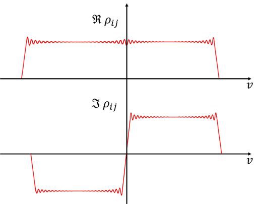
| Fig. 2.34 Real and imaginary part of a frequency power spectrum for an idealized rectangular bandpass. |
In continuum observations the correlation of the signals is usually measured for zero time lags, meaning that the correlation of the measured signal is averaged over the bandwidth, which is defined via a bandpass. In spectral line observations (see Chapt. 3 Sect. 4), measurements at different frequencies across the bandpass are required, which can be implemented by correlating the signals as a function of time lags. After Fourier transforming this correlation output, this yields the so-called cross power spectrum. This cross power spectrum is obtained for  frequency channels (for more detailed information see Chapt. 3 Sect. 4).
To calibrate an interferometer over the bandpass, which represents the filter characteristics of the last IF stage, a continuum point source is used to determine the complex gains of the interferometer, which yields the true cross-correlation spectrum of the observed target source. For calibrator sources with a constant continuum spectrum over the bandpass, the behavior of the complex gains and across the bandpass  are given by the correlated power as a function of frequency for each interferometer of the observing array. The real and imaginary parts of this correlated power, measured for a continuum source with a flat spectrum, are shown in Fig. 2.31 for an idealized rectangular bandpass.
The observed visibility of an unknown target source is given by
![\displaystyle V_\text{ij}^\text{obs}(\nu) = f(\nu)\star\left[g_\text{i}(\nu)\cdot g_\text{j}^\star(\nu)\cdot V(\nu)\right]\,\text{,}](https://wuecampus.uni-wuerzburg.de/moodle/filter/tex/pix.php/7297e6737b5dd7ac508e7e663b3eff7b.gif "\displaystyle V_\text{ij}^\text{obs}(\nu) = f(\nu)\star\left[g_\text{i}(\nu)\cdot g_\text{j}^\star(\nu)\cdot V(\nu)\right]\,\text{,}")
in which ") is the Fourier transform of the truncating function in the frequency domain, which is a sinc function given by
is the Fourier transform of the truncating function in the frequency domain, which is a sinc function given by
 = \frac{\sin(\pi\cdot\nu\cdot K/\Delta\nu)}{\pi\cdot\nu}\,\text{.}")
Here,  is given by a convolution with , since the cross-correlation has only a finite maximum lag of
  . The observed visibility
  of a calibrator source with
  and
and  is then given by
![\displaystyle V_\text{ij}^\text{cal}(\nu)= f(\nu)\star\left[g_\text{i}(\nu)\cdot g_\text{j}^\star(\nu)\right]\,\text{.}](https://wuecampus.uni-wuerzburg.de/moodle/filter/tex/pix.php/ae8aea962d1fb5efc776eeae15172263.gif "\displaystyle V_\text{ij}^\text{cal}(\nu)= f(\nu)\star\left[g_\text{i}(\nu)\cdot g_\text{j}^\star(\nu)\right]\,\text{.}")
Finally, the true visibility  of the observed target source is given by
![\displaystyle V_\text{ij}^\text{true}(\nu) = \frac{V_\text{ij}^\text{obs}(\nu)}{V_\text{ij}^\text{cal}(\nu)} = \frac{f(\nu)\star\left[g_\text{i}(\nu)\cdot g_\text{j}^\star(\nu)\cdot V(\nu)\right]}{f(\nu)\star\left[g_\text{i}(\nu)\cdot g_\text{j}^\star(\nu)\right]}\,\text{,}](https://wuecampus.uni-wuerzburg.de/moodle/filter/tex/pix.php/a8f767a1bf856a6926838936f2d61110.gif "\displaystyle V_\text{ij}^\text{true}(\nu) = \frac{V_\text{ij}^\text{obs}(\nu)}{V_\text{ij}^\text{cal}(\nu)} = \frac{f(\nu)\star\left[g_\text{i}(\nu)\cdot g_\text{j}^\star(\nu)\cdot V(\nu)\right]}{f(\nu)\star\left[g_\text{i}(\nu)\cdot g_\text{j}^\star(\nu)\right]}\,\text{,}")
in which the gains do not cancel out, due to the convolution. Therefore, the original frequency power spectrum, shown in Fig. 2.31, is convolved with the sinc function , due to the finite lag, which will lead to large errors, if the target source has a spectral line near  . This is known as Gibbs' phenomenon.
Since the cross-correlation function has a complex power spectrum, Gibbs' phenomenon has strong influence on the imaginary part of the true visibility, because of the ratio in the equation for , which leads to non-negligible errors, especially for strong line emission near the step at . Since the step in the imaginary part is large, these errors have a strong effect on the phases, producing strong ripples.