Lecture - Fundamental Concepts

As already seen in Chapt. 2 Sect. 4.2, the sensitivity of radio-interferometrical measurements depends on the effective area of the telescopes $A_\text{eff}$ and the bandwidth $\Delta \nu_\text{IF}$. The larger $\Delta \nu_\text{IF}$, the higher the sensitivity. However, using a large bandwidth is problematic, since the Fourier relation between brightness distribution and visibility is only valid for monochromatic signals. Therefore, the effects of the finite bandwidth on the images obtained from radio-interferometrical observations, especially the inevitable effect called bandwidth smearing or chromatic aberration, will be investigated in this section, following the textbook of Taylor et al. (1999).

For a single observing frequency $\nu_0$ the brightness distribution is given by

$\displaystyle \tilde{B}(\xi,\eta) = \int_{-\infty}^{\infty}\int_{-\infty}^{\infty}\tilde{V}(u_0,v_0)\cdot \text{e}^{2\pi\text{i}\cdot(u_0\xi+v_0\eta)}\text{d}u_0\text{d}v_0\text{,}$

in which the "~" indicates the influence of a bandpass. The frequency-independent coordinates $u_0$ and $v_0$ are given by

$\displaystyle \begin{array}{rcl} u_0 = \frac{\nu_0}{\nu}u & \text{and} & v_0 = \frac{\nu_0}{\nu}v \text{,} \end{array}$

where $u$ and $v$ are the actual spatial coordinates of the visibility at the frequency $\nu$.

Therefore, using the generalized similarity theorem for Fourier transformations in $n$ dimensions, which reads

$\displaystyle \mathcal{FT}^n[f(\alpha\vec{x})] = \frac{1}{|\alpha|^n}\cdot F\left(\frac{\vec{s}}{\alpha}\right)\text{,}$

the two-dimensional Fourier relation between visibility and brightness distribution is given by

$\displaystyle B(\xi,\eta)=B\left(\xi_0\frac{\nu_0}{\nu},\eta_0\frac{\nu_0}{\nu}\right)\Leftrightarrow\left(\frac{\nu}{\nu_0}\right)^2\cdot V\left(u_0\frac{\nu}{\nu_0},v_0\frac{\nu}{\nu_0}\right)=\left(\frac{\nu}{\nu_0}\right)^2\cdot V(u,v)\text{.}$

Furthermore, since the smeared visibility $\tilde{V}(u_0,v_0)$ is obtained by rescaling and weighting the true visibility $V(u,v)$ by a normalized bandpass function $G_\text{n}(\nu')$, where $\nu'=\nu-\nu_0$, and then integrating over the frequency band, another important effect must be taken into account. There will be a delay error of

$\displaystyle \Delta\tau=\frac{u_0\xi+v_0\eta}{\nu_0}$

for signals arriving from a direction $(\xi,\eta)$ at frequency $\nu$. Therefore, the phase is shifted by

$\displaystyle 2\pi(\nu-\nu_0)\Delta\tau=2\pi\nu'\frac{u_0\xi+v_0\eta}{\nu_0}$

and the smeared visibility is given by

$\displaystyle \tilde{V}(u_0,v_0)=\int_{-\infty}^{\infty}V\left(u_0\frac{\nu}{\nu_0},v_0\frac{\nu}{\nu_0}\right)\left(\frac{\nu}{\nu_0}\right)^2G_\text{n}(\nu')\text{e}^{2\pi\text{i}\frac{\nu'}{\nu_0}(u_0\xi+v_0\eta)}\text{d}\nu'\text{.}$

For simplicity, a point source with unit amplitude located at $(\xi_0,0)$ is assumed without restricting generality. Then, the true visibility is given by

$\displaystyle V(u,v)=\text{e}^{-2\pi\text{i}u\xi_0}$

and the smeared visibility reads

$\displaystyle \tilde{V}(u_0,v_0)=\int_{-\infty}^{\infty}\text{e}^{-2\pi\text{i}u_0\frac{\nu}{\nu_0}\xi_0}\left(\frac{\nu}{\nu_0}\right)^2G_\text{n}(\nu')\text{e}^{2\pi\text{i}\frac{\nu'}{\nu_0}(u_0\xi+v_0\eta)}\text{d}\nu'\text{.}$

Furthermore, assuming that the bandwidth is sufficiently small, so that $(\frac{\nu}{\nu_0})^2\approx1$ (in practice, $0.95\lesssim(\frac{\nu}{\nu_0})^2\lesssim0.998$), the bandwidth-smeared brightness distribution is given by

$\displaystyle \begin{array}{rl} \tilde{B}(\xi,\eta) & =\int_{-\infty}^{\infty}\left[\int_{-\infty}^{\infty}{e}^{-2\pi\text{i}u_0\frac{\nu}{\nu_0}\xi_0}G_\text{n}(\nu')\text{e}^{2\pi\text{i}u_0\frac{\nu'}{\nu_0}\xi}\text{d}\nu'\right]\text{e}^{2\pi\text{i}u_0\xi}\text{d}u_0\delta(\eta) \\                                                           & =\int_{-\infty}^{\infty}\left[\int_{-\infty}^{\infty}{e}^{-2\pi\text{i}u_0\left(1+\frac{\nu'}{\nu_0}\right)\xi_0}G_\text{n}(\nu')\text{e}^{2\pi\text{i}u_0\frac{\nu'}{\nu_0}\xi}\text{d}\nu'\right]\text{e}^{2\pi\text{i}u_0\xi}\text{d}u_0\delta(\eta) \\                                                                                                                      & =\int_{-\infty}^{\infty}\text{e}^{2\pi\text{i}u_0(\xi-\xi_0)}\left[\int_{-\infty}^{\infty}G_\text{n}(\nu')\text{e}^{2\pi\text{i}u_0\frac{\nu'}{\nu_0}(\xi-\xi_0)}\text{d}\nu'\right]\text{d}u_0\delta(\eta)\text{,} \end{array}$

using $\frac{\nu}{\nu_0}=\frac{\nu_0+\nu-\nu_0}{\nu_0}=1+\frac{\nu'}{\nu_0}$. Here, one can see that the term in squared brackets is the Fourier transform  of the normalized bandpass function over $\nu'$, to an argument $\tau=\frac{u_0}{v_0}(\xi-\xi_0)$ that represents a delay corresponding to the positional offset $\xi-\xi_0$. Therefore, it is helpful to define a delay function $d(\tau)$, given by

$\displaystyle d(\tau) = \int_{-\infty}^{\infty} G_\text{n}(\nu')\text{e}^{2\pi\text{i}\tau\nu'}\text{d}\nu'\text{.}$

Using this delay function, the bandwidth-smeared brightness distribution then reads

$\displaystyle \tilde{B}(\xi,\eta)=\int_{-\infty}^{\infty}\text{e}^{2\pi\text{i}u_0(\xi-\xi_0)}d(\tau)\text{d}u_0\delta(\eta)\text{.}$

Therefore, the bandwidth-smeared brightness distribution is the Fourier transform over $u_0$ of the product of the true visibility with the delay function. Using the convolution theorem, the brightness distribution is given by

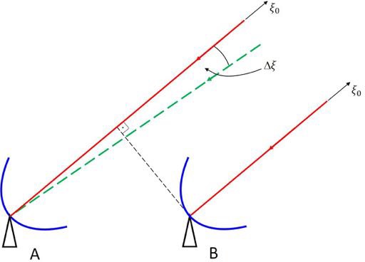
Fig. 2.33 Illustration of the effect of bandwidth smearing. Two signals that arrive from slightly different directions, $\xi_0$ and $\xi_0-\Delta\xi$, with slightly different frequencies can positively interfere, if their delay difference matches.

$\displaystyle \tilde{B}(\xi,\eta)=\int_{-\infty}^{\infty}\text{e}^{2\pi\text{i}u_0(\xi-\xi_0)}\text{d} u_0\delta(\eta) \star \int_{-\infty}^{\infty}d(\tau)\text{e}^{2\pi\text{i}u_0 \xi}\text{d} u_0\text{,}$

which is the convolution of the true image with a position-dependent bandwidth distortion function $D(\xi)$, which is the Fourier transform of the delay function

$d(\tau)$ over $u_0$. Since this distortion function varies with the radial distance $\xi_0$ from the phase center and is always oriented along the radius to the phase center, the final image of an extended source can be interpreted as a radially-dependent convolution. 

The effect of finite bandwidth is illustrated in Fig. 2.30. Here it is assumed that the observed emission of a source at position $\xi_0$ positively interferes exactly at frequency $\nu_0$.  A signal from a neighboring position shifted by $\Delta\xi$ with respect to $\xi_0$ measured by one telescope at a frequency deviating from $\nu_0$ by an amount of $\Delta\nu/2$, for example, can then also produce maximum interference with a signal from $\xi_0$ measured by the other telescope at frequency $\nu_0$, if the delay difference matches. Therefore, a source observed with finite bandwidth can also produce structures away from its nominal position. 

This finite bandwidth effect cannot be removed, because it is described by a mathematical functional. However, there are two methods to minimize the effects of bandwidth smearing. The first method is to limit the field size by dividing the observed area into subfields and produce separate images for all such subfields. To cover the complete area, the images of the subfields can then be fitted together. This technique is called mosaicing. The second method is to split the full frequency band into narrower sections, which will be summed up after imaging each individual data set. This method is called bandwidth synthesis.