Lecture - Image Processing

The range of brightness in astronomical images is often extremely wide, but important features in them often span a very narrow range of brightness (or a span too great for the limited range of displays). Point operations are simple but powerful tools to clearly display information that is locked inside an image. A well-chosen point operation can make hard to see features more visible by changing their original pixel values to a more appropriate range of pixel values. 

Therefore there are two tasks to do:

1. Identifying the numerical range of interest, i.e. isolating the range of pixel values that contain important information (endpoint specification)
   
2. Altering the pixel values for optimum display, i.e. convert old pixel values to a new range (transfer function) 

Methods of endpoint specification

The first step in deciding how to remap the pixel values in an image is to determine the range of useful pixel values (endpoints). Values less than the low endpoint are saturated black, and those greater than the high endpoint are saturated white. Therefore you have to inspect the image and decide the pixel values that will be displayed as black and white. The image histogram allows a quick look at their distribution. Histograms are the key to understand how the value of the pixels that make up an image are distributed over the total range of values available (see Fig. 3.8). The number of pixels is often plotted on a logarithmic scale to visualize the hole range of possible values. 

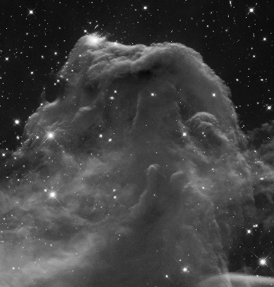
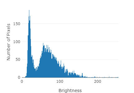
Fig. 3.8: Left: Black and white image of the Horsehead Nebula, Image Credit: NASA, ESA & Hubble Heritage Team (AURA/STScI). Right: corresponding intensity histogram (brightness on a scale 0...255).

Instead of selecting specific pixel values (direct endpoint specification) you can also specify what percentage of pixels is allowed to saturate to black and white (histogram endpoint specification). The principle advantage of the latter is that it is result-oriented. You specify the result you want, therefore results are predictable. In addition, the size of the image and the number of the gray levels in the image do not influence the output. The same fraction of pixels is saturated black, and white, regardless of the image itself. Hence, well-chosen histogram endpoint specifications produce dependable and repeatable results for each type of image.  

Transfer Functions 

Once the high and low pixel values that bracket the range of useful information in an image are determined, the transfer function controls what happens to the pixel values between those limits. Transfer functions are basic techniques that help you change the brightness scale of an image to display information about included features clearly. They are mathematical relationships between old \( (p) \) and new pixel values \( (q) \) :

\( f(p) = q \)

The function is embodied in the operator \( f \). It acts like a black box. When you put the value \( p \) into the black box, the value \( q \) is computed according to the function's formula. It corresponds to a mathematical operation that should be applied to the input values to produce the desired output values.  

Graphically the transfer function is usually shown as the so called transfer curve (see Fig. 3.9). The plotted line shows the relationship embodied in the transfer function. It depicts the mathematical relation between original pixel value \( p \) and new pixel value \( f(p) \). Original pixel values lie between the pixel value in the image that displays as black and the value that displays as white.

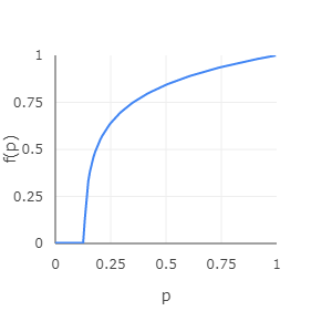
Fig. 3.9: The transfer curve is the graph of a logarithmic transfer function (brightness on a scale 0...1). It depicts the mathematical relationship between original pixel values \( p \) and new pixel values \( f(p) \). 

There are a lot of different transfer functions. The only constraint is that for each old pixel value, there must be only one new pixel value, e.g. the transfer function must be single-valued. Their usage depends on the original image and which imprinted information/features you want to emphasize/display. The most common ones are the linear, logarithmic, gamma and inverse linear (negative) transfer function. We will discuss them in more detail in the following sections.

Transfer functions can help increasing the contrast, and in turn, use more of the available range of brightness values that are shown on the screen or the printout. Changing the range of pixel values is called normalization, dynamic range expansion, or histogram stretching, since the corresponding image brightness histogram becomes stretched and compressed to create a new distribution of pixel values.

Especially when working with large images, i.e. a large number of pixels whose values have to be calculated each time for the new image, it is advantageous to use a look-up table for pixel values and their corresponding transformed values. In case of only 256 brightness values in a simple black and white image, the table of 256 rows has to be computed one time and then only looked up within a loop over all image pixels. This is considerably faster for larger image sizes.