Lecture - Image Processing
| الموقع: | WueCampus |
| المقرر: | vhb - Imaging in Astronomy Demo |
| كتاب: | Lecture - Image Processing |
| طبع بواسطة: | Gästanvändare |
| التاريخ: | السبت، 4 يوليو 2026، 5:58 PM |
جدول المحتويات
- 1. Data Formats and Imaging Software (unavailable)
- 2. Basic Methods I: Pixels (unavailable)
- 3. Basic Methods II: Image operations
- 3.1. What is an Operation?
- 3.2. Geometric Operations - Translation
- 3.3. Geometric Operations - Rotation
- 3.4. Geometric Operations - Scaling
- 3.5. Geometric Operations - Mirroring
- 3.6. Resampling
- 3.7. Point Operations
- 3.8. Negative Transfer Function
- 3.9. Linear Transfer Function
- 3.10. Log Transfer Function
- 3.11. Gamma Transfer Function
- 3.12. Histogram Specification
- 3.13. Image Arithmetic
- 3.14. Image Arithmetic II
- 3.15. Image Arithmetic III
- 4. Illustrating Color (unavailable)
- 5. Linear / Non-Linear Filters and Convolution (unavailable)
- 6. Image Calibration (unavailable)
1. Data Formats and Imaging Software (unavailable)
Learning Objectives:
- How to store the raw data.
- Overview over the most important image-file types and their differences
-
Basic introduction into FITS-files (The Astronomer`s Standard)
-
What kind of imaging software is used in astronomy?
!!! Please note !!!
The content of this section is not part of the Demo-Version!
The content of this section is not part of the Demo-Version!
2. Basic Methods I: Pixels (unavailable)
Learning Objectives:
- What is the difference between a physical and digital pixel?
- What kind of information is stored in a pixel?
- Quantities that describe a pixel's value in an ensemble of pixels.
- What can be illustrated by a image histogram?
!!! Please note !!!
The content of this section is not part of the Demo-Version!
The content of this section is not part of the Demo-Version!
3. Basic Methods II: Image operations
Learning Objectives:
- An image as a histogram, properties and applicable operations.
- The image as a matrix of pixels.
- Transforming the pixel matrices: geometric operations.
- Applying arithmetic to images.
- Displaying image brightness using transfer functions.
3.1. What is an Operation?
Any transformation of an image that starts with the original image and ends with an altered version that concerns pixel value and position can generically be called an operation. Basically, operations can be divided into transformations that change the array of the image pixels but not their value, and consequently transformations that change the values themselves. In certain cases both types are present, for example when an image is shifted along one image axis by a non-integer number of pixels. In this case, new pixel values need to be calculated when the old coordinate system is mapped onto the new one.
Now, that we have seen how basic pixel manipulation works we want to apply certain transformations to the entire array of pixels, i.e. the image itself. Simple transformations such as geometric processes like translation or rotation can be expressed relatively easily by translating pixel positions.
More complex processes like the change of scaling of the pixel value from linear to logarithmic or the subtraction of two images can also be performed pixel-wise. However, an image can also be understood as a matrix that can be altered by another matrix, called the operator, or kernel. In section 5 "Linear/Non-linear Filters" we will see that this formulation allows for the easy usage of operators or filters, that smooth, sharpen, contrast, or gray scale the image by convolving the operator matrix with the original image.
For this part of the lecture basic knowledge of matrix algebra is assumed.
3.2. Geometric Operations - Translation
The most simple geometric transform is the translation along one of the image axis or all at once. An image, or the ensemble of pixels that are translated in the coordinate system, undergo the equations:
\( x' = x + x_T \)
\( y' = y + y_T \)
where \( x' \) and \( y' \) are the coordinates of a pixel \( P \) in the new image and \( x \) and \( y \) the coordinates of the original. The distance of which \( P \) is translated in every direction is denoted by \( x_T \) and \( y_T \), respectively. Figure 3.1 shows two examples of a translation in both directions. Usually, the order in which both translations are performed is arbitrary. In reality the boundary conditions of the image or coordinate system need to be taken into account in every step. One translation may easily shift pixels over the edge of the coordinate system, leading to a loss of information.
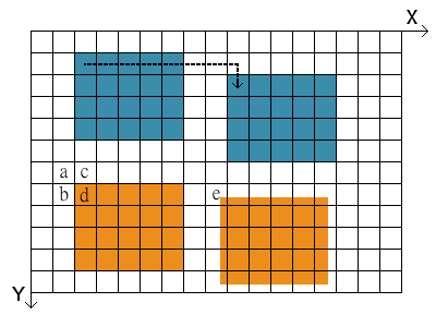
Fig. 3.1: Translation of image by an integer number of pixels (blue images), and non-integer number (orange images).
The translation of an image with an integer number of pixels is not always this case however. What if the translation in Fig. 3.1 is not 8 pixels to the right and 1 pixel down, but for example 7.52 right and 0.74 down? A new pixel value needs to be calculated, where the new one would be (but can't be since the coordinate system does not allow it). In order to do that we need to perform an interpolation of the pixel value. In doing this, we calculate the weighted average of the four pixels that are surrounding the point in the old image. This new value is then assigned to the new pixel in the translated image.
The weighting of all surrounding pixels in the old image (pixels named a, b, c, and d in Fig. 3.1) is done by using the fractional contribution of each pixel, measured by the distance to the point. Have a look at the new image that is transferred by non-integer numbers (orange). One of the former pixels without value (white) now has a bit of orange in it (pixel named e). Consequently, we need to calculate the weighted mean for this pixel, which will become only a bit orange. The new image gets blurred out at the edges as a result of the non-integer translation.
If we want to write a program that translates an old image into a new one by applying a certain instruction, we need to work "backwards". The equations for the translation need to be set up so that the new image can be constructed by referring to pixels of the old image. The translation of an image into a new one is done pixel by pixel. If more than one pixel is needed for the calculation of the value of a new pixel in the new image, like interpolation, it is much more advantageous to start with a new pixel and refer to one or more old pixels.
The procedure of interpolation is necessary whenever the grid of the new pixels does not exactly match the old grid. Besides non-integer pixel translation this will occur in similar applications, i.e. rotation, scaling, and resampling.
3.3. Geometric Operations - Rotation
In order to match an image to another image or coordinate system with different orientation it needs to be rotated. With the rotation angle \( \theta \) the equations for the new coordinates of a pixel are described by:
\( x' = x \cos \theta - y \sin \theta \)
\( y' = x \sin \theta + y \cos \theta \)
in a counterclockwise rotation. In an analogous formulation, the position of every pixel \( (x',y') \) in the new image can be written as a vector and the rotation matrix:
\( \begin{bmatrix} x' \\ y' \end{bmatrix} = \begin{bmatrix} \cos \theta & -\sin \theta \\ \sin \theta & \cos \theta \end{bmatrix} \begin{bmatrix} x \\ y \end{bmatrix} \)
In this simple case the point of rotation \( (x_0, y_0) \) is the point of origin of the coordinate system \( (0,0) \). Quite more useful and practical is the rotation around a certain point of the image or the center of the image, as depicted in Fig. 3.2. In order to rotate a pixel at \( (x, y) \) around an arbitrary point \( (x_0, y_0) \) the equations become:
\( x' = x_0 + (x - x_0) \cos \theta + (y - y_0) \sin \theta \)
\( y' = y_0 - (x - x_0) \sin \theta + (y - y_0) \cos \theta \)
The only pixel that does not move from its position is the pixel at \( (x_0, y_0) \) itself. Again, if the new image is being calculated form the old one, the equations that describe the rotation need to be solved for \( x \) and \( y \), i.e. the inverse transform is needed. The values of all pixels of the rotated image need to be interpolated from the pixel values of the old image in most cases. Therefore, equations for \( x \) and \( y \) that access the values of all four (old) surrounding pixels at the position of the new pixel are required.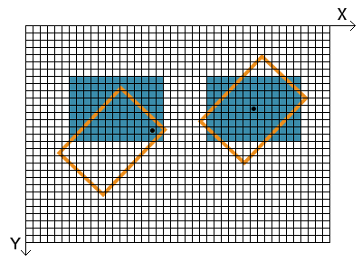
Fig. 3.2: Rotation of an image. The black dots indicate \( (x_0, y_0) \), the center of rotation in each case.
3.4. Geometric Operations - Scaling
Changing the size of an image is also called scaling. This may be done for increasing or decreasing size, respectively. Assuming an equal image scaling of both axes the process can be expressed in its most basic form via:
\( x' = s \, x \)
\( y' = s \, y \)
with the scale factor \( s \). The coordinate of every point is multiplied with the same factor.To scale points relative to a coordinate set \( (x_0, y_0) \), which may be for example \( (0, 0) \) or the middle of the image, the equations become:
\( x' = x_0 + s(x - x_0) \)
\( y' = y_0 + s(y - y_0) \) .
Again, for computing the new and scaled image we must use the equations that are solved for \( x \) and \( y \) in order to obtain all contributions of surrounding pixels in the old image that is mapped onto a new grid. Scaling an image up with an integer factor always results in the best image quality since no interpolation is necessary. Non-integer transformations require interpolation and result in a slightly smoothed image. The figure below shows on the right hand side an example of scaling the factor 2 and the point \( (x_0,y_0) \) in the top left corner of the image. The left hand side shows the scaling up with a factor close to 1. This results in visible image artifacts that come from the interpolation of four pixels of the old image in most cases whereas some pixel values are taken entirely from the old image. In the example below, the scaling also results in a smoothed out edge on two sides.
Fig. 3.3: Scaling of an Image. Left: scale factor close to 1, Right: scale factor 2.
3.5. Geometric Operations - Mirroring
The mirroring of an image is a simple operation that switches the position of pixels in an image on the left/right or top/bottom part, also called "flop" and "flip", respectively. Flopping reverses the X-axis, whereas flipping reverses consequently the Y-axis. Both operations together produce an image that is the same as the original image that has been rotated by 180°.
This circumstance is of particular interest for astronomers since some telescopic systems (like a simple Newton telescope) produce such a reversed image. Applying a flip and flop to the observed image reverses the image to its real format. The usage of a zenith mirror in front of the ocular or CCD sensor on the telescope just mirrors the image in one axis, which is easily corrected after.
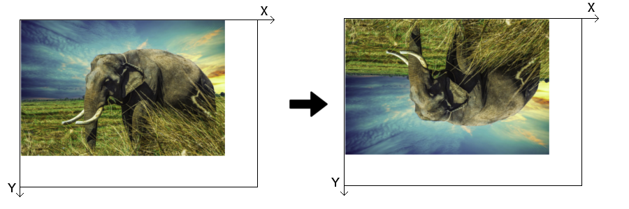
Fig. 3.4: Y-axis mirror or flip.
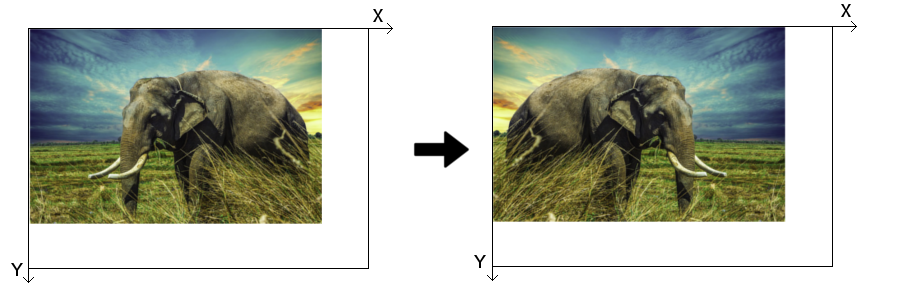
Fig. 3.5: X-axis mirror or flop.
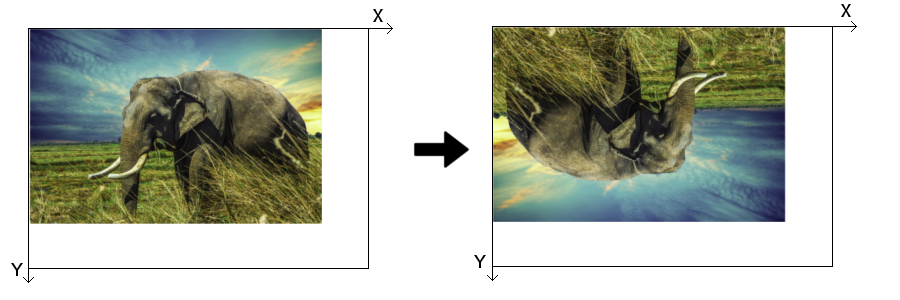
Fig. 3.6: X-axis and Y-axis mirror.
One has to take into account that the simple reversal of coordinates will place the new image outside of the old image. If the image needs, for example, to be mirrored along the Y-axis, the new image also needs to be translated by the height of the image:
\( x' = x \)
\( y' = y_{max} - y \)
Since the operations only deal with integer coordinates and the boundaries of the new image (usually) equal the boundaries of the old image no interpolation is necessary.
3.6. Resampling
Images with limited resolution (so to speak every image) are the result of the measurement with a camera of limited resolution. Usually, the number of pixels in X- and Y-direction is the same as the number of pixels in the physical detector (in optical and X-ray astronomy). When an image of low resolution is taken it seems "blocky" and point-like objects turn into squares. A method that is used to make such an image more life-like with little loss of image information is a process called resampling. Increasing the image resolution is achieved by supersampling, decreasing it by subsampling.
The effect of the resampling in the sense of supersampling is a smoothing of the image. The resolution is being increased via the interpolation of the values of the pixels between the "real" pixels of the original image. We have already seen how interpolation works when applying geometric transformations. This time however, pixels are not simply mapped onto a new grid but a large number of new pixels are inserted in between. Like previously the value of the new pixels is calculated via the fractional contribution of all four neighboring original pixels.
The figure below shows a photograph taken of Saturn's moon Tethys by the Cassini orbiter. The left version is of low quality with pixels of visible size. The version on the right hand side was supersampled and consequently smoothed out.
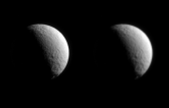
Fig. 3.7: Saturn's moon Tethys. Resampling of a "blocky" image (left) to a more smoothed out version (right). Image Credit: NASA / JPL-Caltech / Space Science Institute, cropping and alterations to pixel size by M. Langejahn.
3.7. Point Operations
The range of brightness in astronomical images is often extremely wide, but important features in them often span a very narrow range of brightness (or a span too great for the limited range of displays). Point operations are simple but powerful tools to clearly display information that is locked inside an image. A well-chosen point operation can make hard to see features more visible by changing their original pixel values to a more appropriate range of pixel values.
Therefore there are two tasks to do:
- Identifying the numerical range of interest, i.e. isolating the range of pixel values that contain important information (endpoint specification)
- Altering the pixel values for optimum display, i.e. convert old pixel values to a new range (transfer function)
Methods of endpoint specification
The first step in deciding how to remap the pixel values in an image is to determine the range of useful pixel values (endpoints). Values less than the low endpoint are saturated black, and those greater than the high endpoint are saturated white. Therefore you have to inspect the image and decide the pixel values that will be displayed as black and white. The image histogram allows a quick look at their distribution. Histograms are the key to understand how the value of the pixels that make up an image are distributed over the total range of values available (see Fig. 3.8). The number of pixels is often plotted on a logarithmic scale to visualize the hole range of possible values.
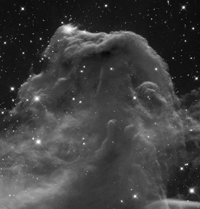
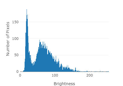
Fig. 3.8: Left: Black and white image of the Horsehead Nebula, Image Credit: NASA, ESA & Hubble Heritage Team (AURA/STScI). Right: corresponding intensity histogram (brightness on a scale 0...255).
Instead of selecting specific pixel values (direct endpoint specification) you can also specify what percentage of pixels is allowed to saturate to black and white (histogram endpoint specification). The principle advantage of the latter is that it is result-oriented. You specify the result you want, therefore results are predictable. In addition, the size of the image and the number of the gray levels in the image do not influence the output. The same fraction of pixels is saturated black, and white, regardless of the image itself. Hence, well-chosen histogram endpoint specifications produce dependable and repeatable results for each type of image.
Transfer Functions
Once the high and low pixel values that bracket the range of useful information in an image are determined, the transfer function controls what happens to the pixel values between those limits. Transfer functions are basic techniques that help you change the brightness scale of an image to display information about included features clearly. They are mathematical relationships between old \( (p) \) and new pixel values \( (q) \) :
\( f(p) = q \)
The function is embodied in the operator \( f \). It acts like a black box. When you put the value \( p \) into the black box, the value \( q \) is computed according to the function's formula. It corresponds to a mathematical operation that should be applied to the input values to produce the desired output values.
Graphically the transfer function is usually shown as the so called transfer curve (see Fig. 3.9). The plotted line shows the relationship embodied in the transfer function. It depicts the mathematical relation between original pixel value \( p \) and new pixel value \( f(p) \). Original pixel values lie between the pixel value in the image that displays as black and the value that displays as white.
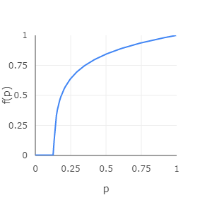
Fig. 3.9: The transfer curve is the graph of a logarithmic transfer function (brightness on a scale 0...1). It depicts the mathematical relationship between original pixel values \( p \) and new pixel values \( f(p) \).
There are a lot of different transfer functions. The only constraint is that for each old pixel value, there must be only one new pixel value, e.g. the transfer function must be single-valued. Their usage depends on the original image and which imprinted
information/features you want to emphasize/display. The most common ones are the linear, logarithmic, gamma and inverse linear (negative) transfer function. We will discuss them in more detail in the following sections.
Transfer functions can help increasing the contrast, and in turn, use more of the available range of brightness values that are shown on the screen or the printout. Changing the range of pixel values is called normalization, dynamic range expansion, or histogram stretching, since the corresponding image brightness histogram becomes stretched and compressed to create a new distribution of pixel values.
Especially when working with large images, i.e. a large number of pixels whose values have to be calculated each time for the new image, it is advantageous to use a look-up table for pixel values and their corresponding transformed values. In case of only 256 brightness values in a simple black and white image, the table of 256 rows has to be computed one time and then only looked up within a loop over all image pixels. This is considerably faster for larger image sizes.
3.8. Negative Transfer Function
This basic example of a transfer function simply assigns every pixel their negative value. Areas of high intensity become dark and vice versa. Since pixel values run on a certain range (0-255 in our case) the "mirroring" of their value is being performed according to their maximum value:
\( f(q) = p_{max} - p \)
Everyone who has used an analog camera at some point knows that exposing a photographic film to the light creates a negative. Not so long ago astronomers used large photographic plates, which worked in the same way. An advantage of using negatives in astronomy is that faint details are more visible to the eye compared to the positive. Differences between two light shades is easier to spot than for two dark shades.
For this and the following examples of applicable transfer functions we are going to use the black and white picture of the Horsehead Nebula, pictured below. It's wide range and non-uniform distribution of brightness demonstrates very well the capabilities of the different functions.

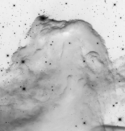
Fig. 3.9: Black and white image (left) and negative (right) of the Horsehead Nebula, Image Credit: NASA, ESA & Hubble Heritage Team (AURA/STScI)
3.9. Linear Transfer Function
The simple but very useful linear transfer function assigns every original pixel value a new value on a linear scale. The endpoints of the function which determine what value is white ( \( p_{white} \) ), and what black ( \( p_{black} \) ) (initially 255 and 0) can, however, be altered. The transfer is described by:
\( f(p) = 0 ~ , ~ p \leq p_{black}\)
\( f(p) = (p-p_{black}) / (\frac{p_{white} - p_{black}}{p_{max}}) ~ , ~ p_{black} < p < p_{white}\)
\( f(p) = p_{white} ~ , ~ p > p_{white}\)
where \( p \) denotes the individual pixel value and \( p_{max} \) the maximum pixel value on the used intensity scale (always 255 for our brightness scale). Pixel values lower than \( p_{black} \) are drawn as black and values higher than \( p_{white} \) white.
Narrowing the band further and further lets certain areas of the image become entirely black or white. Information is lost either way. Completely white areas look over-exposed, because the maximum viable value has been reached. Information in the completely black areas vanishes, because we set a certain threshold value, or sensitivity in a practical sense, below which no values register.
So why even use a linear transfer if information might only get lost? The entire output intensity range (all the different shades of gray) is applied to a more narrow band. This way the contrast in a certain intensity band increases and subtle details and soft gradients become visible.
Move the sliders on the right hand side of the picture below. Observe how narrow windows of allowed pixel values create high contrasts in different bands. The plot shows the transfer function, i.e. the input and output pixel values, respectively. Note that the pixel values are displayed on a scale of 0...1 instead of 0...255.
3.10. Log Transfer Function
A property of astronomical measurements in image form is often a high range of information values, i.e. the brightness of every pixel. The logarithmic scaling allows us to compress the information of an image with pixel values that run from a few to several orders of magnitude higher into a more readable and intuitive form.
Did you know...?
The human eye and brain percieve light intensity strongly non-linear and almost logarithmic. This enables us to see in a wide range of lighting conditions. Mechanical light detectors on the other hand count photons in a linear fashion. In order to replicate an astronomical image "how we would see it" a log transfer function needs to be applied.
The human eye and brain percieve light intensity strongly non-linear and almost logarithmic. This enables us to see in a wide range of lighting conditions. Mechanical light detectors on the other hand count photons in a linear fashion. In order to replicate an astronomical image "how we would see it" a log transfer function needs to be applied.
The corresponding transformation is given as follows. In order to match \( p_{max} \) it is necessary to scale the range of values in the logarithm:
\( f(p) = p_{max} (\frac{Log(p - p_{black})}{Log(p_{white} - p_{black})}) \)
Like before, pixel values smaller than \( p_{black} \) will be depicted as 0, and value greater than \( p_{white} \) as \( p_{max} \). The image in the example below seems overall brighter since the pixel values in the middle of the range are relatively enhanced compared to very low and very high values of \( p \). Increasing the value for \( p_{black} \) only a bit quickly separates the fainter regions in darkening them substantially. The real strength of the logarithmic transfer function is the reduction of a large value range (such as a nebula in a field of bright stars) of more than 256 steps in the applications here. Real images, as measured in astronomical observations, often feature millions of steps, depending on how many photons have been measured in a pixel.
3.11. Gamma Transfer Function
A powerful and more flexible tool than the previous point operation is given by the gamma transfer function. Basically, it allows to brighten or darken the middle tones of an image without much change at the end points, i.e. very dark and very bright tones. The function takes advantage of the scale of 0 ... 1, whose endpoints, that are connected by a smooth curve, remain constant when applying a power to all brightness levels / tones \( p \). A power of 1 leaves the curve as a straight line. When the power is greater 1, the curve bows upward, if it is less than 1, it bows downward. The middle tones of the image become more pronounced or less pronounced, respectively. The darkest and brightest tones do not change significantly. The transfer function is defined as:
\( f(p) = p^{1/\gamma} \)
where \( p \) is between 0 and 1. Consequently, the standard brightness values of 0 ... 255 need to be scaled accordingly. The convention of using \( 1/\gamma \) instead of \( \gamma \) simply makes the using the parameter \( \gamma \) more intuitive: increasing \( \gamma \) also increases the middle tones.
Like in the examples before, all pixel values lower that \( p_{black} \) will be set to 0, and all values greater than \( p_{white} \) to \( p_{max} \). The pixel values between \( p_{black} \) and \( p_{white} \) are to be transferred onto the range of 0 ... 1, raised to the power \( 1/\gamma \), and finally transferred onto the range of 0 ... \( p_{max} \) :
\( f(p) = p_{max} (\frac{p - p_{black}}{p_{white} - p_{black}})^{1/\gamma} \).
The gamma transfer function is efficient for highlighting weak or diffuse objects in an image, like nebulae or super nova remnants. Alternative methods like narrowing the brightness band ( \( p_{black} \) to \( p_{white} \) ) or using the Log transfer function may throw away information, or may only be useful when the image brightness encompasses several orders of magnitude.
3.12. Histogram Specification
Images are characterized by a certain intensity distribution, i.e. the intensity histogram (that often has an uneven shape). Astronomical images have in many cases an abundance of dark tones and few bright ones, representing the background with a few bright stars here and there, respectively. We have already seen that a manually applied transfer function can help increasing the contrast and, in turn, use more of the available range of brightness values that are shown on the screen or the printout. But, what if we want to go a step further and not only change the dynamic range and / or contrast of the image but the intensity distribution itself in order to suppress or promote different intensity levels? The process of histogram specification makes exactly this possible. Often also named histogram matching or histogram stretching, this method does exactly what it says: stretching the image intensity histogram via a certain transfer function so that the resulting histogram of the new image resembles the desired distribution. We will look at several examples of some distributions which are usually applied for deep-sky objects or lunar images.
The process works as follows. Below each step a python code sample is provided.
1) Compute the intensity histogram \(h(p)\) and the corresponding cumulative histogram \(h\_sum(p)\) of the original image, with \(p\) being the pixel value. On a programming level, these histograms are simply represented by arrays with the length of 256 for a standard 8-bit grayscale image. Each value indicates the histogram height at that brightness value (0...255).
# build histogram h
for y in range(0, ymax-1):
	for x in range(0, xmax-1):
		p = image(x,y)
		h[p] = h[p] + 1
# build cumul. histogram h_sum
for i in range(0, 255):
	h_sum[i] = h_sum[i] + h[i]
2) Generate a target histogram \(th(p)\), i.e. the desired shape of the intensity histogram of the transformed image. For this to happen we apply a transfer function \(a(p)\), which can be a for example a Gaussian distribution. The target histogram becomes
\(th(p) = a(p/256)\)
for a function that runs from 0...1. This operation is executed within a loop over all pixel values.
# build target histogram th
# call a target function, use a Gaussian function here
for i in range(0, 255):
	th[i] = gaussian[i/256]
3) Compute the cumulative target histogram \(th\_sum(p)\). Note that the sums of both cumulative histograms are different. To make them equal, each element in \(th\_sum(p)\) must be multiplied with the ratio of the sums. Both cumulative histograms are now identical, except the distribution of pixel values.
# build target cumul. histogram th_sum
for i in range(0, 255):
	th_sum[i] = th_sum[i] + th[i]
# make sums of cumul. target histograms equal
ratio = h_sum[255] / th_sum[255]
for i in range(0, 255):
	th_sum[i] = th_sum[i] * ratio
4) Determine the look-up table (LUT) which lets \(h\_sum(p)\) track \(th\_sum(p)\) (the LUT is used in the next step as a transfer function for the pixel values of the original image). The process works as follows: a loop runs over every pixel value and calculates LUT(\(p\)), i.e. at every pixel value (0...255) the algorithm compares \(h\_sum(p)\) and \(th\_sum(p)\). If the value at the target histogram is larger that the original histogram LUT(\(p\)) we define a new pixel value \(p\_new\) (initially 0) that increases by 1. The value increases until the image histogram count matches the target histogram count. If the target histogram is smaller that the original image histogram \(p\_new\) stays the same. At the end of each iteration we set the LUT(\(v\)) equal to \(p\_new\).
# create LUT that makes the cumul. histogral track the target cumul. histogram
p_new = 0
for i in range(0, 255):
	while th_sum[p_new] < h_sum[i]
		p_new = p_new + 1
	LUT[i] = p_new
5) Apply LUT to image. With the previous step done we have defined out transfer function that carries out the histogram specification. We apply the transfer function to the image at every pixel coordinate and obtain the new image.
# apply LUT
for y in range(0, ymax-1):
	for x in range(0, xmax-1):
		image_new(x,y) = LUT(image(x,y))
The transformation of the original image simply applies the LUT to determine the target pixel value in the new image. The histograms of the newly created images are often characterized by odd-looking gaps between the histogram bars. This is due to the fact that a certain interval of intensities in the original have a limited number of gray levels. The algorithms that determines the LUT skips certain target pixel values until the target catches up with the original.
Especially deep-sky images profit from histogram specification. The histogram of a typical deep-sky image, like in the example below, has a sharp peak at low intensity, corresponding to the dark background. The second component is a peak with exponential tail that describes the object itself. Some frequently used functions \(a\) in image processing that dictate the target histogram are for example:
- Flat-line / constant histogram, also called histogram equalization. The target histogram is a flat line, and the cumulative histogram consequently a wedge shape:
\(h(x) = c\),
where \(c\) is a constant. Because of its simplicity we list this function here, although it has limited use for deep-sky imagery. Many pixels that are originally dark or in the middle of the intensity scale are pushed to high intensities, letting the image look bright and washed-out. Images with a bi-modal histogram, like dark backgrounds and very bright objects (e.g. planets) are seemingly transformed into a over-exposed variant with gray backgrounds and extremely bright objects.
- Gaussian shape. This distribution assumes a variation of tones around a central mean. However, astronomical images often feature an exponential decline towards high intensities. Consequently, a Gaussian distribution that is shifted somewhat towards low intensities produces the most realistic and very effective images. The corresponding function is
\(h(x) = \frac{1}{\sigma \sqrt{2\pi}} e^{-\frac{1}{2}(\frac{x-\overline{x}}{\sigma})^2} \),
with the base of natural logarithms \(e\), the standard deviation \(\sigma\), and the mean value \(\bar{x}\) of \(x\).
- Exponential fall-off. Although many astronomical images appear like this histogram shape, they actually have low numbers of pixels at very low intensity values. Transforming the shape into a true exponential function lets many dark pixels appear even darker, if not black. However, images of bright extended objects display greater detail in the faint outer parts after applying this function, described by
\(h(x) = e^{-kx}\),
where \(k\) is a constant value.
Below we see the familiar image of the Horsehead Nebula. Apply the different versions of histogram specification and observe how the image and the corresponding histograms and cumulative histograms are changing.
3.13. Image Arithmetic
Simple mathematical operators like addition or subtraction, and involving two images of equal dimensions, are the foundation of a multitude of further image processing like calibration, comparison, or combination. At this point we are looking at only two images that are involved in the usage of one operation. Image math includes addition, subtraction, multiplication, and division of each one of the pixels of one image with the corresponding pixel of the other image. In the following examples the result of every operation will be a new image itself.
The addition of two images stacks the value of every pixel in image A with the corresponding pixel of image B. Consequently, the image gets brighter. Depending on the maximal allowed pixel value that is used, this operation might result in saturated pixels of the new image, i.e. white pixels that have reached the maximum value. This will lead to information loss and should be avoided if possible. The whole resulting image can for example be re-normalized, so that the brightest pixel equals the maximum allowed value and all other pixels are scaled accordingly. The example below is not adjusted for this case.
Subtracting two images works analogously. In a similar way, the resulting values may lie outside the allowed range of pixel values. This will be the case when one image is subtracted from another with lower pixel values. Here, it is advantageous to add a certain constant value to the equation (the whole image). The example below shows what happens when two images that are in parts almost identical get subtracted from one another. We add the constant value of 150 to every pixel of image A and then perform the subtraction by image B. Subtle differences in the background can be seen as soft lines and shapes in the resulting image. This is expected for nearly identical images with e.g. slightly different exposure times. The darker areas of the cup in the middle even become a bit darker (value 0) since they (very dark tones plus 150) are then indeed over-subtracted. The gray lines across the cup are the result of the subtraction of a light tone (dark cup in image A + 150) with a dark tone (dark lines in image B). The cup on the right side in the resulting image also features gray lines, which are brighter compared to the cup in the middle since the cup is brighter itself.
A special case of the subtraction of two image is the absolute difference. Here, no adding of a constant is necessary to fully preserve the conveyed information. The absolute value of the difference highlights missing objects, especially those whose brightness value is rather different compared to the area at its position in the other image. Consequently, the black cup in the middle notably stands out. A large part of the cup to the right is not highlighted very strongly, since the brightness of the pixels in its center areas is roughly that of the background in image A. The shadow of the cups in the middle and to the right are also highlighted because of the large difference in brightness to the background. Because our perception of brightness partially depends on the brightness of the surrounding areas, the difference in images is not always intuitive. Subtraction and absolute difference as image operations serve as effective tools in finding even subtle changes.
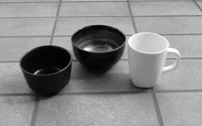
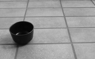
Fig. 3.14: Image A (left) and image B (right)
3.14. Image Arithmetic II
The multiplication of two images can for example be used to highlight ranges of brightness in an image. This can be done by using a sequence of multiplications to create a discontinuous transfer function. Another useful application is the masking of an image, i.e. the multiplication of a normal image with an image whose values are only 0 or 1. This way sections of the original image are cut away (or painted black) by multiplying them with 0 and the remaining sections with 1. Multiplication must be normalized to produce resulting images with pixel values in the range of 0 ... 1. After the multiplication the values are scaled back to their original range (e.g. 0 ... 255). In the example below, the result becomes a bit darker than the images A and B, since values in the range of 0 ... 1 are multiplied with each other. The pixel values of the bright cup on the right are reduced significantly, leading to the "ghostly" appearance in front of the background. The new pixel values are determined as follows:
\( p_A(x,y)' = p_A(x,y) / p_{max} \)
\( p_B(x,y)' = p_B(x,y) / p_{max} \)
\( p_{A \cdot B}(x,y) = p_A(x,y)' \cdot p_B(x,y)' \cdot p_{max}\)
As with multiplication, the division of two images needs to be normalized to the range 0 ... 1. Dividing images is also an effective and sensitive tool for highlighting differences between the images. However, the operation can prove challenging since the result spans a wide range of values and the division by 0 (black pixels) is undefined. In this case we limit the resulting pixel value to \( p_{max} \) (white). After normalizing image A and B same as for the multiplication process, the division is done by:
\( p_{A/B}(x,y) = p_A(x,y)' / p_B(x,y)' \cdot p_{max}\)
In the example below we perform the operation B/A. This especially highlights the cup in the middle, because the background in image B is divided by the relatively dark pixel values of the cup itself.
Fig. 3.15: Image A (left) and image B (right)
3.15. Image Arithmetic III
In this example we can see how useful the application of simple arithmetic operations on scientific image data is. Below there are two photographs of globular cluster M3. These astronomical objects contain variable stars which can alter their visible magnitude within short periods of time. Both images show photographs just a few hours apart.
Did you know...?
Globular clusters are among the oldest astronomical objects in our galactic neighborhood and are composed of tens of thousands of stars (if not more) in a spherical shape. The Milky Way galaxy itself harbors more than a hundred globular clusters within its outer regions, the so-called halo. The population of stars in these objects differs significantly from stars in the host galaxy, in the sense that their chemical composition features far less elements heavier than hydrogen and helium.
Globular clusters are among the oldest astronomical objects in our galactic neighborhood and are composed of tens of thousands of stars (if not more) in a spherical shape. The Milky Way galaxy itself harbors more than a hundred globular clusters within its outer regions, the so-called halo. The population of stars in these objects differs significantly from stars in the host galaxy, in the sense that their chemical composition features far less elements heavier than hydrogen and helium.
Adding the images results in a brightened version with a seemingly denser center. This effect is produced by adding very bright pixel values (the light gray area between the visible stars) on top of very bright values until the value reaches the maximum and becomes white.
The subtraction of both images (A-B) reveals a far more interesting picture. Like before, we add an artificial offset of 150 to the resulting pixel values. This enables us to see pixels that would have a resulting value of less than 0 with no offset. Information would be lost. These black pixels (black stars) represent a negative difference of both images, i.e. pixels that are brighter in image B compared to image A. In the same way, white pixels (white stars) in the resulting image represent stars that are brighter in image A compared to B. With this simple tool it is possible to pinpoint variable stars between two measurements and associate brightening or fainting with each object.
Similarly, the absolute difference of both images shows all variable objects as white dots, albeit without the information whether the individual object is brightening or fainting.
Multiplying both images with each other acts like a slight reduction of brightness. Since the multiplication of all pixel values is normalized, the effective pixel values in the multiplication are between 0 and 1 (all values are divided by 255). Multiplying the pixel values results in a even lower value than before, like 0.7 * 0.68 = 0.467. The last step is multiplying the result with 255 to get the actual pixel value. In this example: 178 * 173 -> 119. This reduction of brightness is stronger for pixels of lower value. Therefore, there not only a reduction of brightness in the resulting image, but also slightly higher contrast.
The division of image B by A creates a very bright result. In this example, the images A and B are almost identical, which leads to, or very close to values of 1 (white) when dividing two nearly equal pixel values. The pattern of black squares in the top left corner is due to areas in image B that already have zero intensity. The blocky appearance of the pattern is due to compression artifacts of the image. Compressed images, are (mostly) divided into smaller rectangular parts with an individual brightness value assigned to them. Individual areas that correspond to variable stars can be made out when switching back and forth between the abs difference and the divide button.
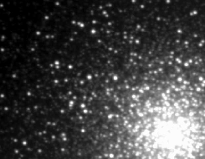
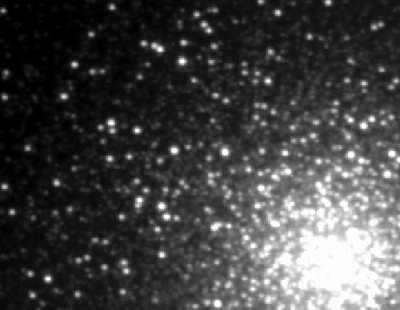
Fig 3.16: Globular Cluster M3, two different photographs A (left) and B (right) within a single night, Credit: J.D.Hartman
Learning Quiz - Image Operations
Go to the following quiz to test what you have learned in this section, or select the quiz from the main course site.
Go to the following quiz to test what you have learned in this section, or select the quiz from the main course site.
Tutorial - Image Operations
Go to the corresponding tutorial to try some image operations by yourself, or select the tutorial from the main course site.
Go to the corresponding tutorial to try some image operations by yourself, or select the tutorial from the main course site.
4. Illustrating Color (unavailable)
Learning Objectives:
- Color components of an image
- RGB and CMY palette.
- Color conversion to Grayscale
- True, false, and representative color
!!! Please note !!!
The content of this section is not part of the Demo-Version!
The content of this section is not part of the Demo-Version!
5. Linear / Non-Linear Filters and Convolution (unavailable)
Learning Objectives:
- image filters as linear and non-linear operators
- convolution in 1D and 2D
- unsharp masking
- application of filters to images
- edge detection
!!! Please note !!!
The content of this section is not part of the Demo-Version!
The content of this section is not part of the Demo-Version!
6. Image Calibration (unavailable)
Learning Objectives:
- Why is image calibration necessary?
- What are the regions of possible light-matter interactions?
- What effects influence our primary astronomical signal?
- How can we handle this influences?
- How does the callibration change for different wavelength?
!!! Please note !!!
The content of this section is not part of the Demo-Version!
The content of this section is not part of the Demo-Version!