Numpy & Scientific Programming: Moving from lists to arrays
Data Science heavily relies on Linear Algebra. While Python is a flexible multi-purpose programming language it isn't necessarily fast in doing numerical operations.
Numpy was developed to alleviate this drawback and offers various functions to perform mathematical operations efficiently.
Essentially, it provides you with three things:
np.ndarray: A flexible datatype for storing sequences of numbers in a fixed shape of any form.- Prebuilt function to manipulate
np.ndarrays - An extensive set of mathematical operations directly applicable on
np.ndarrays
Also, Numpy became the foundation of most other data science libraries in Python, rendering it the lingua franca between different libraries or even inspiring other libraries like PyTorch to borrow many of its concepts.
First things first - Numpy: Usage basics
Installation
Numpy is a third-party library and is not included in a standard Python installation.
To install it open a terminal, and type pip install numpy or conda install numpy depending on your Python setup
Import
By convention, the whole numpy is imported with the abbreviation np.
import numpy as np
Creating ndarrays
There are many ways to create arrays.
Here is a quick overview over the most common ones:
- Creating from existing (nested) lists
import numpy as np
my_list = [[1, 2], [3, 4]]
my_array = np.array(my_list)
print(my_array)
[[1 2]
 [3 4]]
- Creating arrays with fixed content
zero_array = np.zeros(shape=(2, 2))
print(zero_array)

ones_array = np.ones((2, 2))
print(ones_array)

constant_array = np.full(shape=(2, 2), fill_value=-100)
print(constant_array)
[[0. 0.]
 [0. 0.]]
[[1. 1.]
 [1. 1.]]
[[-100 -100]
 [-100 -100]]
np.zeros(shape=(3, 2))
array([[0., 0.],
       [0., 0.],
       [0., 0.]])
- Creating arrays with consecutive content
numbers = np.arange(9)
numbers
array([0, 1, 2, 3, 4, 5, 6, 7, 8])
rand_normal_array = np.random.randn(10000)
print(rand_normal_array.shape)
print("Mean:", rand_normal_array.mean(), "Std:", rand_normal_array.std())

rand_integer_array = np.random.randint(0, 2, (10))
print(rand_integer_array)
(10000,)
Mean: 0.0011282100385092903 Std: 1.0016185642357456
[0 0 0 1 1 0 0 1 0 0]
ndarray: Dimensionality
Creating a ndarray from a nested list, gives you a multidimensional arrays.
In theory, ndarrays can have as many dimensions as you like.
Since arrays have a fixed size, each dimension also has a fixed length.
The number of dimension and the size of each dimension determine the shape of an array.
There are might be special naming conventions depending on the shape of your arrays:
- 1-dim => Vector
- 2-dim => Matrix
Note: Obviously in a mathematical sense, these terms have more implications but we ignore those for now.
ndarray: Indexing
Like lists, you can also use indexing or slicing to address unary values or certain patches of your data.
The syntax mostly follows Python`s conventions but is extended to directly address specific dimensions.
array = np.arange(27).reshape(3, 3, 3)
print(array.ndim)
print(array.shape)
print(array)
3
(3, 3, 3)
[[[ 0  1  2]
  [ 3  4  5]
  [ 6  7  8]]

 [[ 9 10 11]
  [12 13 14]
  [15 16 17]]

 [[18 19 20]
  [21 22 23]
  [24 25 26]]]
# Get the first element across all dimensions
print(array[0, 0, 0])

# Get the first "matrix"
print(array[0, :, :])

# Get the last row vector of the second matrix
print(array[1, -1, :])
0
[[0 1 2]
 [3 4 5]
 [6 7 8]]
[15 16 17]
# How to get number 17?

array[1, 2, 2], array[1, -1, -1]
(17, 17)
To index or slice with ndarrays you can specify values for each dimension independently.
It's also possible to combine slicing and indexing at specific dimensions.
Values for dimension are written into one single slicing expression, value are separated by commas.
array[<dim0>, <dim1>, <dim1>, ...]
ndarray: Masking
Masking allows you to select all values in an array which fulfill a condition.
Let's generate some data mimicking the number of hourly visits for a webpage over a year.
site_traffic = np.random.randint(100, 1000, (365, 24))
site_traffic.shape, site_traffic.mean()
((365, 24), 549.8228310502283)
Suppose we would like to count the hours with high traffic (> 750 visits).
The Pythonic way to do this would be to treat the array as a nested list and iterate over all the dimensions using for-loops:
high_traffic_hours = 0
for day_idx in range(site_traffic.shape[0]):
    for hour_idx in range(site_traffic.shape[1]):
        traffic = site_traffic[day_idx, hour_idx]
        if traffic > 750:
            high_traffic_hours += 1
high_traffic_hours
2382
But there is a better way to do this, using numpy masking functionality.
Masking is a technique to create a boolean mask that has the same shape as the original array.
The mask identifies values in the array that meet a specified condition, marking them as True while marking other values as False.
high_traffic_periods = site_traffic > 750
high_traffic_periods
array([[ True, False, False, ..., False,  True, False],
       [ True, False, False, ..., False, False, False],
       [ True, False, False, ..., False, False, False],
       ...,
       [ True, False, False, ..., False, False,  True],
       [False,  True, False, ...,  True,  True,  True],
       [False, False, False, ..., False,  True, False]])
Because boolean values translate to 0, 1, we can easily sum them up, to get the number of high-traffic hours.
high_traffic_periods.sum()
2382
We can also use masks, to perform:
- Retrieving Values
- Inplace operations
Retrieving
high_traffic_values = site_traffic[high_traffic_periods]
print(high_traffic_values)
print(high_traffic_values.shape)
[776 762 903 ... 903 929 876]
(2382,)
Inplace Manipulations
low_median_traffic = site_traffic.copy()
low_median_traffic[high_traffic_periods] = 0.0
low_median_traffic
array([[  0, 100, 470, ..., 334,   0, 734],
       [  0, 616, 241, ..., 257, 205, 300],
       [  0, 502, 320, ..., 275, 634, 481],
       ...,
       [  0, 194, 441, ..., 194, 393,   0],
       [176,   0, 364, ...,   0,   0,   0],
       [161, 661, 121, ..., 472,   0, 440]])
ndarray: Reshaping
It's possible to change the shape of an existing array.
This operation is called reshaping. Reshaping works by specifying the new number and sizes of dimensions.
To make reshaping work the number of entries in the newly created array has to match the number of entries in the existing array.
vector = np.array([1, 2, 3, 4, 5, 6, 7, 8])
print(vector)
print("Orig shape:", vector.shape)
print("No. of entries:", vector.size)

matrix = vector.reshape(2, 4)
print(matrix)
print("New shape:", matrix.shape)
print("No. of entries:", matrix.size)

tuples = vector.reshape(-1, 2)
print(tuples)
print("New shape:", tuples.shape)
print("No. of entries:", tuples.size)
[1 2 3 4 5 6 7 8]
Orig shape: (8,)
No. of entries: 8
[[1 2 3 4]
 [5 6 7 8]]
New shape: (2, 4)
No. of entries: 8
[[1 2]
 [3 4]
 [5 6]
 [7 8]]
New shape: (4, 2)
No. of entries: 8
The .reshape-method takes in as many arguments as desired dimensions, and each argument specifies the number of entries in that dimension.
It's possible to leave the size of one dimension and just write -1, numpy will infer the size automatically.
ndarray: Computations
Numpy offers a wide variety of functions that are optimized to work efficiently on ndarrays.
These functions take in either a single array or two of them and return an output-array.
# Average hourly visits
site_traffic.mean(), np.mean(site_traffic)
(549.8228310502283, 549.8228310502283)
As you can see above, unary-functions can often (but not always) directly be accessed as a property of the ndarray.
Some of these function can also be applied along a specific dimension:
# Average number of visits per day
site_traffic.mean(axis=1).shape
(365,)
Binary functions work like the math operators you all know:
a, b  = np.arange(3), np.arange(3) * 2
a, b
(array([0, 1, 2]), array([0, 2, 4]))
# Element wise addition
c = a + b
c
array([0, 3, 6])
import matplotlib.pyplot as plt


# Define the angle of rotation in radians
theta = np.pi/9
# Create a 2D rotation matrix
rotation_matrix = np.array([[np.cos(theta), -np.sin(theta)],
                            [np.sin(theta), np.cos(theta)]])

points = np.array([
    [1, 1],
    [0, 0]
])

plt.scatter(x=points[:, 0], y=points[:, 1])
plt.grid(True)
plt.show()

# Matrix multiplication to rotate points in space
points_rotated = rotation_matrix @ points.T
# Equivalent to:
# points_rotated = np.matmul(rotation_matrix, np.transpose(points))


plt.scatter(x=points_rotated[:, 0], y=points_rotated[:, 1])
plt.grid(True)
plt.show()


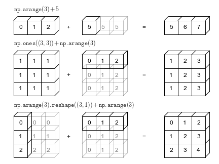
ndarray: Broadcasting
As we've seen now numpy is fast in processing ndarrays of the same shape.
This does not only apply to vectors or matrices but also to arrays of arbitrary dimensionality
But, it is also possible to perform arithmetic operations, with ndarrays and scalar values.
point_shifted = points + 2
plt.scatter(x=point_shifted[:, 0], y=point_shifted[:, 1])
plt.grid(True)
plt.show()

It is also possible to compute with arrays of different shapes under some circumstances:
matrix = np.arange(9).reshape(3, 3)
print(matrix)

row_vec = np.array([1, -1, 5])
print(row_vec)
print("matrix + row_vec=\n", matrix + row_vec)

col_vec = np.array([[1], [-1], [5]])
print(col_vec.shape)
print(col_vec)
print("matrix + col_vec=\n", matrix + col_vec)
[[0 1 2]
 [3 4 5]
 [6 7 8]]
[ 1 -1  5]
matrix + row_vec=
 [[ 1  0  7]
 [ 4  3 10]
 [ 7  6 13]]
(3, 1)
[[ 1]
 [-1]
 [ 5]]
matrix + col_vec=
 [[ 1  2  3]
 [ 2  3  4]
 [11 12 13]]
To perform those operations on ndarrays with mixed dimensionality, numpy uses broadcasting to automatically adjust the dimensions of the array with fewer dimensions, by padding it to the right size.
Source: https://jakevdp.github.io/PythonDataScienceHandbook/02.05-computation-on-arrays-broadcasting.html
To successfully perform broadcasting some constraints on the shape and size of the arrays have to be fulfilled:
for dim_a, dim_b in zip(a.shape[::-1], b.shape[::-1]):
    if not (1 in (dim_a, dim_b) or dim_a == dim_b):
        raise ValueError("operands could not be broadcast together")
If arrays do not have the same number of dimensions the array with fewer dimensions is expanded by adding dimensions to the left.
(np.([1]).unsqueeze(0) => np.ndarray([[1]]))
Pandas: Wrangling with data in Python
While Numpy is designed to work with data in arbitrary shapes, Pandas is optimized to work with tabular data.
DataFrame
Like Numpy's ndarray, there is one essential container class which builds the core of the library, the DataFrame.
Conceptually, you can think of a DataFrame as the Python version of a Spreadsheet.
Consider, the sales table from above:
| Transaction_ID: int | Product: str | Price: float | Quantity: int |
|---|---|---|---|
| 0 | Beer | 0.89 | 6 |
| 0 | Chips | 1.99 | 1 |
| 1 | Milk | 1.20 | 3 |
| 2 | Bread | 2.55 | 1 |
| ... | ... | ... | ... |
It can directly be represented as a DataFrame:
import pandas as pd

columns = ["Transaction", "Product", "Price", "Quantity"]

data = [
    [0, "Beer", 0.89, 6],
    [0, "Chips", 1.99, 1],
    [1, "Milk", 1.20, 3],
    [2, "Bread", 2.55, 1],
]

df = pd.DataFrame(data=data, columns=columns)
df
| Transaction | Product | Price | Quantity | |
|---|---|---|---|---|
| 0 | 0 | Beer | 0.89 | 6 |
| 1 | 0 | Chips | 1.99 | 1 |
| 2 | 1 | Milk | 1.20 | 3 |
| 3 | 2 | Bread | 2.55 | 1 |
DataFrame consists of columns and rows.
Typically each column represents a feature, or field of your data. And each row represents a represents a record/ instance of your dataset.
df.shape, df.columns, df.index
((4, 4),
 Index(['Transaction', 'Product', 'Price', 'Quantity'], dtype='object'),
 RangeIndex(start=0, stop=4, step=1))
Pandas offers a wide variety of different way to access your data:
# Access columns
df["Price"]
0    0.89
1    1.99
2    1.20
3    2.55
Name: Price, dtype: float64
# Access rows
df.loc[0]
Transaction       0
Product        Beer
Price          0.89
Quantity          6
Name: 0, dtype: object
Also there is a wide variety of additional functions to manipulate your data, or create new aggregated views on it:
# Sorting based on specific columns
df.sort_values(by="Price", ascending=False)
| Transaction | Product | Price | Quantity | |
|---|---|---|---|---|
| 3 | 2 | Bread | 2.55 | 1 |
| 1 | 0 | Chips | 1.99 | 1 |
| 2 | 1 | Milk | 1.20 | 3 |
| 0 | 0 | Beer | 0.89 | 6 |
# Aggregating all rows with a specific value
df.groupby("Transaction")["Price"].sum()
Transaction
0    2.88
1    1.20
2    2.55
Name: Price, dtype: float64
df.groupby("Product")["Quantity"].mean()
Product
Beer     6.0
Bread    1.0
Chips    1.0
Milk     3.0
Name: Quantity, dtype: float64
# Counting unique values within columns
df.Transaction.value_counts()
Transaction
0    2
1    1
2    1
Name: count, dtype: int64
# Querying for data:
df.query("Price < 2.0")
# Equivalent to
# df[df["Price"] < 2.0]
| Transaction | Product | Price | Quantity | |
|---|---|---|---|---|
| 0 | 0 | Beer | 0.89 | 6 |
| 1 | 0 | Chips | 1.99 | 1 |
| 2 | 1 | Milk | 1.20 | 3 |
df.query("Product.str.startswith('B')")

# Equivalent to
# df[df["Product"].str.startswith("B")]
| Transaction | Product | Price | Quantity | |
|---|---|---|---|---|
| 0 | 0 | Beer | 0.89 | 6 |
| 3 | 2 | Bread | 2.55 | 1 |
def is_even(x):
    return x % 2 == 0

df.query("@is_even(Transaction)")

# Equivalent to
# df[[is_even(t) for t in df["Transaction"]]]
| Transaction | Product | Price | Quantity | |
|---|---|---|---|---|
| 0 | 0 | Beer | 0.89 | 6 |
| 1 | 0 | Chips | 1.99 | 1 |
| 3 | 2 | Bread | 2.55 | 1 |
# Saving data in a variety of commonly used formats
df.to_csv("sales.csv", index=False)
df.to_excel("sales.xlsx", index=False)
# Loading data in various formats
df = pd.read_excel("sales.xlsx")
df
| Transaction | Product | Price | Quantity | |
|---|---|---|---|---|
| 0 | 0 | Beer | 0.89 | 6 |
| 1 | 0 | Chips | 1.99 | 1 |
| 2 | 1 | Milk | 1.20 | 3 |
| 3 | 2 | Bread | 2.55 | 1 |
And so much more!
How to learn really Pandas?
TL;DR Just use it!
Learning Pandas - even more like Numpy - is best done, while you work on your specific projects.
Going through all its features in the course would be too extensive. So we'll introduce additional features as we go on.
You are strongly encouraged to stay curious and always keep on googling (or ask ChatGPT) "How to do xy in Pandas?" 😊
But there are some great resources to start digging deeper: