Demokurs: Introduction to Engineering Mathematics
| Website: | WueCampus |
| Kurs: | vhb - Demokurs Lehramt |
| Buch: | Demokurs: Introduction to Engineering Mathematics |
| Gedruckt von: | Gast |
| Datum: | Samstag, 13. Juni 2026, 22:05 |
Beschreibung
1. Functions


The chapter Functions includes:

- Linear and Quadratic Functions
- Power Functions, Polynomials and Power Series
- The Exponential Function and Growth
- Trigonometric Functions
- Multivariable Functions
- Curves and Maps
- Exercises
1.1. Linear and Quadratic Functions
This chapter contains the definition of the term function and examines linear and quadratic functions.
What is a function?
Example 1.
The following relationship exists between the speed of sound in metres per second, \(c\), and the air temperature in degrees Celsius, \(\theta\): \[c=331,5\cdot\sqrt{1+\frac{\theta}{273}} \qquad \text{for } \theta>-273\] \(c=c(\theta)\) is a function of \(\theta\).
Definition 1: Function
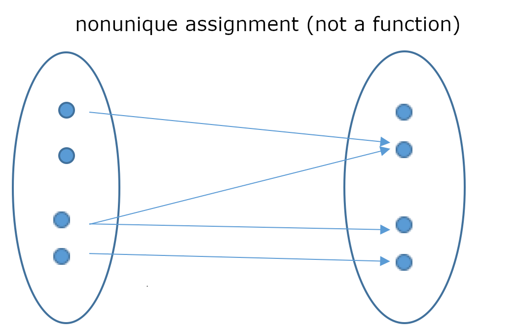
For arbitrary sets \(A\) and \(B\), a function (or map) \(f: A\rightarrow B\) is a rule which assigns a unique value \(y=f(x) \in B\) to \(x \in A\). Here \(A\) is called domain and \(B\) the codomain. The graph of \(f\) is the set \(G_f = \{(x,y) \in A\times B : y=f(x)\}.\)
Explanation: This means that a function is a unique assignment rule.
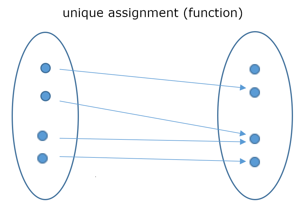
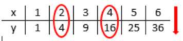
This example, assigns to each natural number \(x\) its square \(y=f(x)=x^2\):
Usually, the functions that are relevant within this course are represented (plotted) as a graph in a coordinate system. A graph is – as defined above – a set of points, which results in the common curve depiction. Those points have the shape \((x|f(x))\).
Linear functions
The functional equation of a linear function \(f:x\in\mathbb{R}\mapsto f(x)\in\mathbb{R}\) can be written as: \[f(x) = m\cdot x + t, \qquad m,t\in\mathbb{R}\]
Here, \(m\) is called the slope or gradient and \(t\) the \(y\)-intercept of the function (more precisely: of the graph of the function).
For a positive slope/ gradient \(m>0\) the line increases (rises), for a negative slope/ gradient \(m<0\) the line decreases (falls). The larger the absolute value of \(m\), the steeper the line rises or falls: The larger a positive gradient is, the steeper the line increases; the smaller a negative gradient is, the steeper the line decreases.
\(m=0\) results in the special case of a line which is parallel to the \(x\)-axis, that is, horizontal: \[f(x)=t\]
One should note that lines parallel to the \(y\)-axis cannot be depicted by linear functions, because the slope would have to be infinitely large. In that case infinitely many values would have to be assigned to one x-value (which would contradict the definition of a function).
Such linear functions can be represented with the following equation (which is not a function!): \[x=a, a\in\mathbb{R}\]As \(t\) increases or decreases the value of the function independently from \(x\) (this means \(t\) does not change for different \(x\) values/ is the same for all \(x\)), we can move the whole graph along the \(y\)-axis. For positive \(t\) the graph moves up and for negative \(t\) it moves down. If \(t=0\), then the line passes through the origin; in this case we have \(f(0)=m∙0+t=t=0\).
Interactivity. Explore the influence of the parameters \(m\) and \(t\) on the linear function.
This notation means that the function rule \(f\) assigns to each value \(x\) (the „pre-image“) a function value \(f(x)\) (the „image“). Both \(x\) and \(f(x)\) lie in \(\mathbb{R}\) in this case.
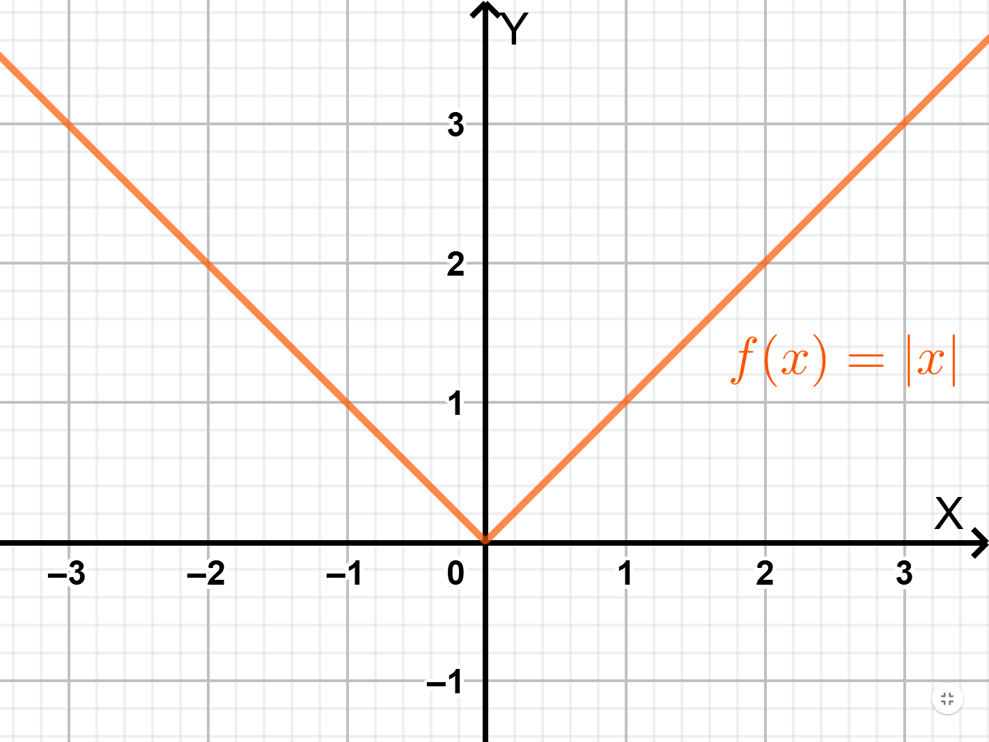
The absolute value \(|a|\) of a number \(a\) is its value without the sign: \[|3|=3\] \[|-3|=3\]
Acccordingly, one can define the absolute value function: \[f(x)=|x|=\begin{cases} x, \text{for } x\geq 0\\ -x, \text{for } x < 0\end{cases}\]
Calculating the gradient and the \(y\)-intercept
The gradient of a linear function is calculated using the so-called 'gradient triangle' as follows: \[m=\frac{\Delta y}{\Delta x} = \frac{\Delta f(x)}{\Delta x} = \frac{f(x_2)-f(x_1)}{x_2-x_1}\]
Here, the vertical distance between two points on the graph is divided by the horizontal distance of those two points (to be more precise, the values of the distances). So, the gradient depicts how the vertical value changes when the horizontal value changes.
As an example, road gradients are measured in a similar way. Here, the difference in altitude covered by the car is measured while it moves 100m in the vertical direction. (So, the actual distance is the hypotenuse of the resulting right-angle triangle) With this in mind - \(x\) as the difference in altitude per 100m - the gradient is expressed as a percentage.

The \(y\)-intercept \(t\) equals the value the function has for \(x=0\), which is calculated by evaluating the function for \(0\): \[t = f(0)\]
Plotting the graph of the function
To plot the graph of the function you should memorize the following steps:
-
Starting at the origin move along the \(y\)-axis until you reach \(t\). We call this point \(P\).
-
Starting at \(P\) move up, vertically, the value of the numerator of \(m\) and move right, horizontally, the value of the denominator of m. We call this point \(Q\).
-
The graph is a straight line through \(P\) and \(Q\).
If \(m\) has already been calculated, \(m\) can be used as the numerator, and \(1\) as the denominator, since \(m=\frac{m}{1}\)
Calculating the angle \(\alpha\) between the straight line and the \(x\)-axis
With the definition for the trigonometric function of the tangent in right-angled triangles ((the length of) the opposite side divided by (the length of) the adjacent side) it is true that: \[tan(\alpha ) = \frac{\Delta f(x)}{\Delta x} = m\]
according to the definition of the gradient m and therefore: \[\alpha = arctan(m)\]
Zeroes
A linear function has exactly one zero (\(f(x) = 0\)), that means there is only one intersection with the \(x\)-axis. The exception being the case where \(m=0\). Here \(f\) is a constant function and thus the graph is a line parallel to the \(x\)-axis: \(f(x) = t\). Such a function does not have a zero for \(t\neq 0\). For \(t=0\) it holds: \(f(x)=0\). In this case the function has infinitely many zeros.
To calculate the zero \(x_0\) set \(f(x_0)=m\cdot x_0+t = 0\) and solve the equation for \(x_0\): \[x_0 = -\frac{t}{m}\]
Relationships between graphs of linear functions
Two lines \(G_f\) and \(G_g\) are parallel if, and only, if their gradients \(m_1\) and \(m_2\) are equal: \[m_1 = m_2 \Leftrightarrow G_f \parallel G_g\]
So, parallel lines \(f_1, f_2, f_3,\ldots \) only differ through their \(y\)-intercepts \(t_1, t_2, t_3,\ldots \) This means the functions emanate from each other through translations (parallel shifts) in the vertical direction (upwards and downwards).
Two lines \(G_f\) and \(G_g\) are perpendicular, if and only if, the product of their gradients \(m_1\) and \(m_2\) equals -1: \[m_1\cdot m_2 = -1 \Leftrightarrow G_f \perp G_g\]

Exercise.
Justify this relationship between \(m_1\) and \(m_2\).
Quadratic functions
The general form of the quadratic function \(f:x\mapsto f(x)\) is: \[f(x) = a\cdot x^2 + b\cdot x + c, \qquad a \neq 0,b,c\in\mathbb{R}\]
Graphs of quadratic functions are parabolas.
The coefficient of \(x^2\) i.e. a, determines the form of the parabola. If \(a\) is a positive number, the parabola opens upwards; if negative, it opens downwards. The bigger the value of \(|a|\) is chosen, the graph appears more closed. Conversely the shape of the parabola becomes less closed for a smaller value of \(|a|\).
A change in the parameter \(c\) shifts the parabola in the \(y\)-direction, because \(c\) is independent from \(x\). As a result changes in \(x\) have no influence on \(c\). If \(c\) is increased by one, the graph is displaced upwards by one. On the other hand if \(c\) is decreased by one, the graph is displaced downwards by one.
\(c\) is therefore basically the \(y\)-intercept which we encountered by looking at straight lines.
\(|a|\) denotes the absolute value of \(a\), that is the value of \(a\) "without the sign".
Identifying vertices
The vertex of the parabola is either the absolute minimum point (if \(a\) is a positive number) or the absolute maximum point (if \(a\) is a negative number). If the function is converted to the vertex form below by completing the square and using the binomial formula, the coordinates of the vertex can be read off directly: \[f(x) = a\cdot (x-x_s)^2 + y_s.\]
With this form of the equation the graph of \(f\) can be seen as a variation of the (standardized) parabola with the form \(g(x)=x^2\). \(f\) generates from this by shifting it to the right by \(x_S\), up by \(y_S\) and by dilation/compression by the factor \(a\).
From the general form of the quadratic equation (see above), we get the coordinates of the vertex as: \[x_s = -\frac{b}{2a}\] \[y_s = \frac{4ac-b^2}{4a}\]
The vertex then has the coordinates \((x_s, y_s)\). The graph is axially symmetric to the line parallel to the \(y\)-axis and passing through \(x_s\).
Exercise.
Show that the general form \(f(x)=ax^2+bx+c,\quad a, b, c\in\mathbb{R}, a\neq 0\) can be converted into the vertex form \(f(x) = a\cdot (x-x_s)^2 + y_s.\)
A turning point is labeled as "absolute" (or global) when it is the largest/smallest value in the whole domain. In contrast a "local" Maximum/Minimum is only a maximum/minimum in a particular area.
The coefficient \(a\) does not change after this transformation!
Roots
A quadratic function has zero, one or two roots, depending on the position of the vertex \(S\) and the sign of \(a\).
To calculate the roots we set \(f(x) = 0\) and solve the equation using the quadratic formula: \[x_{1/2} = \frac{-b\pm\sqrt{b^2-4ac}}{2a}\]
New terms:
-
Function
-
Linear function
-
Quadratic function.
Short revision exercises
Exercise 1.
Calculate the roots of the function f and plot its graph for \(f(x) = -3x + 6\)
Exercise 2.
Let \(P = (4, 3)\) and \(Q = (0, -2)\) be two points. Construct the equation of the straight line g passing through \(P\) and \(Q\) and calculate the angle at which g intersects with the x-axis.
Exercise 3.
Determine the vertex \(S\) of the parabola given by \(f(x) = -5x^2 + 30x + 47\) by completing the square.
Exercise 4.
Calculate the roots of the parabola given by \(f(x) = -\frac{1}{2}x^2+\frac{1}{2}x+3.\)
1.2. Power Functions, Polynomials and Power Series

In this chapter we revise the characteristics of power functions and polynomials. Then, in an optional section, we introduce another analysis concept -- the power series.
Power functions
Definition 1: Power function with positive integer exponent
A power function with a positive integer exponent is a function of the form: \[f : x\mapsto a\cdot x^n \qquad a\in\mathbb{R},\ n\in\mathbb{N},\ D=\mathbb{R}\]
Setting \(n=0\) provides a constant function \(f(x)=a.\)
Note: We have already met two specific examples of power functions in the last chapter: For \(n=1\) we have the pure linear function \(f\) where \(f(x) = ax\) and for \(n=2\) we have the pure quadratic function \(f\) where \(f(x) = ax^2\). Additionally, for \(n=0\) we get the special case of a constant function \(f(x) = a∙x^0 = a∙1 = a\).
Exercise.
Vary the parameter \(a\) on the adjacent example for \(f(x) = a\cdot x^3\). Comment on how the graph changes.
Definition 2: Power function with integer exponents
A power function with an integer exponent is a function of the form: \[f : x\mapsto a\cdot x^z \qquad a\in\mathbb{R},\ z\in\mathbb{Z},\ D=\mathbb{R}\backslash\{0\}\]
They can be separated into two groups, which have opposite characteristics:
-
\(f(x) = a\cdot x^n\) (positive integer exponent, \(n>0\)): These functions have one root at \(x=0\) and grow without bounds for large \(|x|\) (tend towards plus or minus infinity). They are continuous on the whole of \(\mathbb{R}\). Their graphs always have one branch and are called parabolas of order \(n\).
-
\(f(x) = a\cdot x^{-n}\) (negative integer exponent, \(-n<0\)): These functions have a pole at \(x=0\) and approach 0 for large \(|x|\). There are continuous on \(\mathbb{R}\backslash\{0\}\). We call their graphs hyperbole of order \(n\). Because of the pole, they have two branches.
The graphs of power functions with odd exponents are point-symmetric about the origin, while those of power functions with even exponents are axially-symmetric about the \(y\)-axis.
\[f(-x) = (-x)^2 = x^2 = f(x)\]
\[f(-x) = (-x)^3 = -(x^3) = -f(x)\]
Parabolas of order \(n\) - the building blocks of polynomials
For growing \(x\) the absolute value of \(x^n\) increases continuously and diverges towards \(\infty\).
For growing \(x\) the denominator (actually its absolute value) increases and the fraction converges towards \(0\).
Definition 3: Power functions with fractions in the exponents
A power function with a fraction in the exponent is a function of the form: \[f : x\mapsto a\cdot x^{\frac{1}{n}} \qquad a\in\mathbb{R},\ n\in\mathbb{N},\ D=\mathbb{R}^+_0\]
Exercise.
On the right are the graphs of the function \(f\) where \(f(x)=x^{\frac{1}{n}}\) for \(n \in \{2,3,4,5,6\}\). Describe these graphs, paying particular attention to the domain, monotonicity, and the largest and smallest values of the function. Are there points common to all graphs of these functions? Justify this!
Example 1: Root function
A particular example of a power function is the function \[f : \mathbb{R}^+_0\rightarrow\mathbb{R}^+_0, x\mapsto\sqrt{x}=x^{\frac{1}{2}}\] which takes the square root of every positive number. Analogously the \(k\)-th roots \(\sqrt[k]{x}\) are also power functions thanks to the identity \(\sqrt[k]{x}=x^{\frac{1}{k}}.\) The \(k\)-th root function \(f\) where \(f(x)=x^{\frac{1}{k}}\) is the inverse of the power function \(g\) where \(g(x) = x^k\). Also \(g\) is the inverse of \(f\).
Definition 4: Power functions with negative fractions in the exponent
A power function with a negative fraction in the exponent is a function of the form: \[f : x\mapsto a\cdot x^{-\frac{1}{n}} \qquad a\in\mathbb{R},\ n\in\mathbb{N},\ D=\mathbb{R}^+\]
Exercise.
Compare the graphs of the functions with negative fractions in the exponents (blue) with the graphs of the functions that were introduced earlier with positive fractions in the exponents (red dotted). Pay particular attention to the domain, symmetry, monotonicity and the largest and smallest values of the function. Are there points which all graphs have in common? Justify this.
Definition 5: Power functions with rational number exponents
A power function with a rational number exponent is a function of the form: \[f : x\mapsto a\cdot x^{\frac{p}{q}} \qquad a\in\mathbb{R},\ p\in\mathbb{Z},\ q\in\mathbb{N},\ D=\mathbb{R}^+\]
Exercise.
Compare the graphs of power function with rational exponents (blue) with those we met in the above sections (red and purple dotted); by using the scroll bar you can alter the exponents. Describe the similarities and differences of the graphs, paying particular attention to the domain and symmetry.
Power functions with rational number exponents
The representation of functions of the form \(f(x) = (\sqrt[k]{x})^p\) as \(f(x) = x^{\frac{p}{k}}\) plays a role when differentiating functions as the common rules for derivatives are transferred to root-functions.
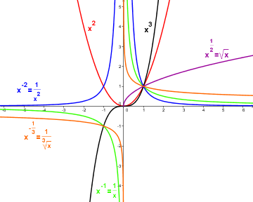
Various power functions.
Polynomials
Polynomials are constructed by adding up power functions \(a \cdot x^n\) where \(n\) is a natural number. They are defined and continuous over the whole of \(\mathbb{R}\).
Definition 6: Polynomial of degree \(n\)
For \(a_0, a_1,\ldots, a_n \in\mathbb{R},\) \[p : \mathbb{R}\rightarrow\mathbb{R}, x\mapsto\sum^n_{k=0}a_kx^k = a_0+a_1^x+a_2x^2+\ldots+a_nx^n\] is called a polynomial of degree \(n\), when \(a_n\neq 0.\)
So, per definition constant, linear, quadratic and power functions are polynomials.
The behaviour of the graphs of polynomials with degree \(>2\) is not as easy to determine as for graphs in special cases like constant, linear and quadratic functions. To determine the characteristics of these polynomials and their graphs, we use the method of curve sketching taught in school (see below).
Various polynomial functions.

New terms:
-
Power function
-
Polynomials
-
Power series
Short revision exercises
Exercise 1.
Sketch the following power functions: \(x^3\), \(x^{\frac{1}{3}}\), \(x^{-3}\), \(x^{-\frac{1}{3}}\)
Exercise 2.
Specify the type and position of the extrema, inflection points and the roots for the polynomial function \[f(x)=-\frac{1}{4}x^4+\frac{3}{2}x^2-2x-2.\]
1.3. The Exponential Function and Growth
In this chapter we meet a particularly important function: the exponential function. Afterwards we categorize the growth of arbitrary functions with the help of the growth of functions we already know.
Introductory example: Linear and exponential growth
Example 1: Growth of capital with simple interest
When using simple interest, the amount of interest added each year to the initial capital (or principal) \(K_0\), is \(K_0\cdot\frac{p}{100}\). The interest in following years is calculated only on \(K_0\). We can therefore assume that the yearly interest is withdrawn by the investor. It can be deduced that the capital after \(n\) years is \[K(n) = K_0 + K_0\cdot\frac{p}{100}\cdot n\]
When using compound interest the interest is paid out on the interest of the preceding years, i.e., the initial capital \(K_0\) is multiplied every year by \((1+\frac{p}{100}).\) It can be deduced that the capital after \(n\) years is \[K(n) = K_0\cdot(1+\frac{p}{100})^n\]
Exercise.
Explain how this formula was derived!
Both formulae for the growth of the capital are valid only for complete years (\(n\in\mathbb{N}\)), as the bank pays interest annually. The graph of the capital is therefore a discrete graph.
By approximation we can also work with the exponent \(x\in\mathbb{R}\), in order to calculate the capital at arbitrary times (e.g., \(x=1.75\) years). The graph of the capital after an arbitrary time period \(x\) is a continuous curve. (This continuous expansion can be switched on and off in the applet to the right using the tick box.)
The growth of capital governed by the functional equation \(K(x) = K_0\cdot(1+\frac{p}{100})^x\) is called exponential growth. Here the independent variable \(x\) is the exponent and this new type of function is therefore called an exponential function.
The general exponential function
Definition 1: Exponential function to the base \(a\)
The function \[f: \mathbb{R}\rightarrow\mathbb{R}, f(x) = a^x = \exp(x\cdot\log(a)) \qquad (a\in\mathbb{R}^+, a\neq 1)\] is called the exponential function to the base \(a\).
Theorem 1: Functional equation
For all \(x,y\in\mathbb{R}\) we have: \[a^{(x+y)}=a^x\cdot a^y\]
Proof. The functional equation follows directly from the theorem of multiplication of two powers with the same basis: \[b^m\cdot b^n = b^{m+n}\]
\(\square\)
Properties of a general exponential function \(x\mapsto a^x\)
-
The exponential function is defined for all \(x\in\mathbb{R}.\)
-
It has only positive output.
-
All exponential functions of the form \(f(x) = a^x\) pass through the point (0,1).
-
For \(0 \lt a \lt 1\) the function \(f(x)\) is monotonically decreasing, for \(a=1\) it is constant and for \(a>1\) monotonically increasing.
-
The graphs of \(f(x) = a^x\) and \(g(x) = a^{-x} = \frac{1}{a^x}\) are symmetric about the \(y\)-axis. For both graphs the \(x\)-axis is a horizontal asymptote.
-
For \(0 < a < 1\) the function \(f(x) = a^x\) is monotonically decreasing, \(f\) diverges for \(x \rightarrow -\infty\) and converges to \(0\) for \(x \rightarrow \infty\).
-
For \(a=1\) \(f\) is constant
-
For \(a > 1\) the function \(f(x) = a^x\) is monotonically increasing. \(f\) diverges for \(x \rightarrow \infty\) and converges to \(0\) for \(x \rightarrow -\infty\).
Interactivity. Explore the behaviour of the exponential function under varying parameters using the Geogebra app.
-
(Exercise on \(x \mapsto a^x\)) Set \(m\) and \(b\) to 1, \(c\) and \(d\) to 0 and vary the value of the base \(a\) using the scrollbar. Describe how the graph changes for different values of \(a\). Verify the properties of the function \(x \mapsto a^x\) given above.
-
Why doesn't the function \(f(x)\) exist for negative \(a\)?
-
(Exercise on \(x\mapsto m\cdot a^x\)) Let \(a\) again be fixed (and non-zero). Describe the effect on the graph by varying \(m\) and find a certain characteristic for certain pairs of numbers.
-
(Exercise on \(x\mapsto a^{b\cdot x}\)) From now on let \(a\) be fixed (and non-zero). Describe the effect on the graph by varying \(b\) and find a certain characteristic for certain pairs of numbers.
-
(Exercise on \(x\mapsto a^x+c\)) Again set \(m\) and \(b\) to 1 and \(d\) to 0 and vary the value of \(c\) using the scroll bar. Describe how the graph changes.
-
(Exercise on \(x\mapsto a^{x+d}\)) Again set the value of \(m\) and \(b\) to 1 and \(c\) to 0 and vary the value of \(d\) using the scroll bar. Describe how the graph changes.
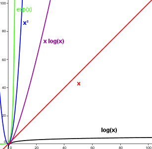
The logarithm - the inverse of the exponential function
The inverse of the exponential function is the logarithm \[\log_a(x): \mathbb{R}^+\rightarrow\mathbb{R}.\] It is continuous and strictly monotonous increasing.
The logarithm function results as the inverse function by rearranging the exponential function: \[y=f(x)=a^x\] Then \[x=f^{-1}(y)=log_a(y)\] To plot the function in the familiar coordinate system the form \(x \rightarrow f^{-1}(x)\) is most commonly used.
Interactivity. Work through the following assignments using the Geogebra app.
-
Vary the value of \(a\) using the scroll bar and describe how the graph changes for different values of \(a\). What do all the functions have in common? What differences are there for different values of \(a\)?
-
What do you notice if you compare the exponential and the logarithmic functions? Describe the position of both graphs in relation to one another.
Theorem 2 (Functional equation)
For all \(x,y\in\mathbb{R}^+\) we have: \[\log_a(x\cdot y)=\log_a(x)+\log_a(y)\]
Proof.
The functional equation follows directly from the functional equation of the exponential function (theorem 1): \[\log_a(x\cdot y) = \log_a(a^{\xi}\cdot a^{\eta}) =\] \[= \log_a(a^{\xi+\eta}) = \xi+\eta = \log_a(x)+\log_a(y)\]
\(\square\)
New terms:
-
Exponential growth
-
Exponential function
-
Logarithm
1.4. Trigonometric Functions
The important characteristics of the trigonometric functions sine \((\sin)\), cosine \((\cos)\), and tangent \((\tan)\) are now to be explained.
The Basics
Trigonometric functions describe relationships between the sides and angles of a right-angled triangle. The side opposite the right angle is called hypotenuse, also identifiable as the longest side of a right triangle in Euclidean geometry. The side opposite an acute angle is called the opposite (side), and the side adjacent to it (that is not the hypotenuse) is called the adjacent (side). Note that the naming depends on which of the two acute angles is chosen. In cases where context doesn't make it obvious, one should distinguish which angle's opposite or adjacent is in question.
One obtains the graphs of these trigonometric functions by plotting the ratio of the corresponding sides (on the \(y\)-axis) against the angle \(\alpha\) in radians (on the \(x\)-axis). These are shown in the figures below.
The trigonometric functions are defined on a right-angled triangle as follows:
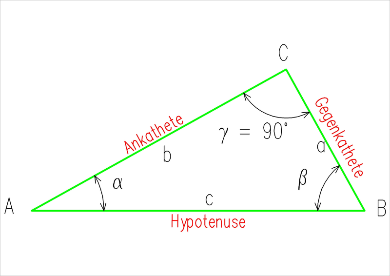
right-angled triangle
Sine
Sine is the ratio of the opposite to the hypotenuse.
Definition: Sine
\[\sin(\alpha)=\frac{\text{opposite}}{\text{hypotenuse}}\]
The term sine comes from the Latin "sinus" meaning arc or curve. Since the hypotenuse is always the longest side, the value of the sine is always smaller than 1.
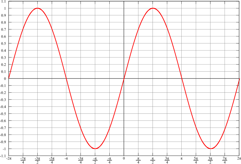
The sine function
Cosine
Cosine is the ratio of the adjacent to the hypotenuse.
Definition: Cosine
\[\cos(\alpha)=\frac{\text{adjacent}}{\text{hypotenuse}}\]
The term Cosine comes from the Latin "complementi sinus", it is the sine of the complementary angle. The value of the cosine is also obviously less than 1, because the hypotenuse is the longest side of the triangle.
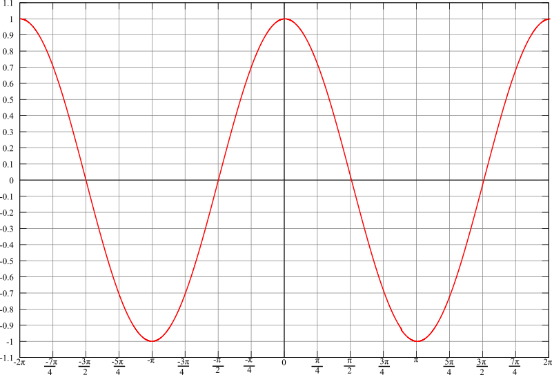
The cosine function
Tangent
Tangent is the ratio of the opposite to the adjacent.
Definition: Tangent
\[\tan(\alpha)=\frac{\sin(\alpha)}{\cos(\alpha)}=\frac{\frac{\text{opposite}}{\text{hypotenuse}}}{\frac{\text{adjacent}}{\text{hypotenuse}}}=\frac{\text{opposite}}{\text{adjacent}}\]
The name tangent comes from the tangent of a unit circle. Details are in the next chapter.
The value of the tangent can easily exceed 1, because on the one hand the hypotenuse does not occur in the quotient (as it did for sine and cosine limiting their value to 1), and on the other hand the adjacent can be smaller than the opposite.
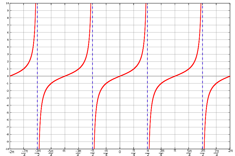
The tangent function
Trigonometry of a unit circle
If we plot a unit circle around the origin in a coordinate system and choose a point \(P\) on the unit circle in the first quadrant, we can draw a right-angled triangle in the unit circle such that the hypotenuse is the line segment connecting the origin and \(P\).
Let \(x\) be the \(x\)-coordinate and \(y\) the \(y\)-coordinate of \(P\). We can consequently determine \(\sin\), \(\cos\) and \(\tan\) using the above definitions. In this case the hypotenuse has the length 1, the values of sine and cosine are: \[\sin(\alpha)=y\qquad\quad\cos(\alpha)=x\]
With the help of Pythagorean theorem we obtain the equation \[\sin^2(\alpha)+\cos^2(\alpha)=1\]
Extend the line segment connecting the origin and \(P\) past \(P\) and draw a line tangent to the circle at the point (1,0) (this runs vertically). The tangent (tan) of the angle is equal to the length of the line segment connecting on the one hand the point of intersection between the line of origin passing through \(P\) and tangent to the circle (that runs vertically in our case) and on the other hand the point (1,0). The term tangent comes from this description.
If we choose the point \(P\) to be on the unit circle but not in the first quadrant then we obtain the values of sine, cosine and tangent for arbitrary angles.
Thereby we obtain the following relationships: \[-\sin(\alpha)=\sin(-\alpha)\qquad\quad\cos(-\alpha)=\cos(\alpha)\]
Hence sine is an odd function (the graph is point-symmetric about the origin), and cosine an even function (the graph is axially-symmetric about the \(y\)-axis). We also find that sine and cosine are periodic functions with period 360\(^{\circ}\) (\(=2\pi\)).
Tangent is likewise periodic, since \[\tan(\alpha+180^{\circ}) = \frac{\sin(\alpha+180^{\circ})}{\cos(\alpha+180^{\circ})} = \frac{-\sin(\alpha)}{-\cos(\alpha)} = \tan(\alpha)\]
Right-angled triangle in the unit circle
General definitions of \(\text{ }\sin\), \(\text{ }\cos\text{ }\) and \(\text{ }\tan\)
More general forms of trigonometric functions \(\sin\), \(\cos\) and \(\tan\) can be given by modifying the basic functions with a number of parameters. Consider functions of the form \[a\ \cdot\ \sin(b\cdot\alpha\ -\ c)\ +\ d\] \[a\ \cdot\ \cos(b\cdot\alpha\ -\ c)\ +\ d\] \[a\ \cdot\ \tan(b\cdot\alpha\ -\ c)\ +\ d.\] Then each of the variables \(a, b, c, d\) has a distinct role, explained below.
Variation of the amplitude
The factor \(a\) changes the displacement in the \(y\)-direction:
| \(a=1\) | the normal function is given |
|---|---|
| \(a<1\) | the amplitude is lower |
| \(a>1\) | the amplitude is greater |
Change of the period
The factor \(b\) changes the period of the function:
| \(b=1\) | the normal function is given |
|---|---|
| \(b<1\) | the period repeats less frequent |
| \(b>1\) | the period repeats more frequent |
Translation in the \(x\)-direction
The factor \(c\) translates the graph in the \(x\)-direction.
| \(c=0\) | the normal function is given |
|---|---|
| \(c<0\) | displacement to the left |
| \(c>0\) | displacement to the right |
Translation in the \(y\)-direction
The factor \(d\) shifts the graph in the \(y\)-direction:
| \(d=0\) | the normal function is given |
|---|---|
| \(d<0\) | displacement downwards |
| \(d>0\) | displacement upwards |
Optional reading: Series definitions of trigonometric functions
The inverse functions of \(\text{ }\sin\), \(\text{ }\cos\text{ }\) and \(\text{ }\tan\)
The inverse functions of \(\sin\), \(\cos\) and \(\tan\) are as follows: \[\arccos: [-1,1]\ \rightarrow\ \mathbb{R}\quad\text{Arccosine}\] \[\arccos(x)\ =\ \cos^{-1}(x)\] \[\arcsin: [-1,1]\ \rightarrow\ \mathbb{R}\quad\text{Arcsine}\] \[\arcsin(x)\ =\ \sin^{-1}(x)\] \[\arctan: \mathbb{R}\ \rightarrow\ \mathbb{R}\quad\text{Arctangent}\] \[\arctan(x)\ =\ \tan^{-1}(x)\]
Some specific values of \(\text{ }\sin\), \(\text{ }\cos\text{ }\) and \(\text{ }\tan\)
| Angle | \(0^\circ\) | \(30^\circ\) | \(45^\circ\) | \(60^\circ\) | \(90^\circ\) | \(180^\circ\) | \(270^\circ\) |
|---|---|---|---|---|---|---|---|
| Radians | \(0\pi\) | \(\frac{\pi}{6}\) | \(\frac{\pi}{4}\) | \(\frac{\pi}{3}\) | \(\frac{\pi}{2}\) | \(\pi\) | \(\frac{3\pi}{2}\) |
| Sine | \(0\) | \(\frac{1}{2}\) | \(\frac{\sqrt{2}}{2}\) | \(\frac{\sqrt{3}}{2}\) | \(1\) | \(0\) | \(-1\) |
| Cosine | \(1\) | \(\frac{\sqrt{3}}{2}\) | \(\frac{\sqrt{2}}{2}\) | \(\frac{1}{2}\) | \(0\) | \(-1\) | \(0\) |
| Tangent | \(0\) | \(\frac{\sqrt{3}}{3}\) | \(1\) | \(\sqrt{3}\) | NaN | \(0\) | NaN |
New terms:
-
Sine
-
Cosine
-
Tangent
-
Trigonometry on the unit circle
-
General definition of \(\sin\), \(\cos\) and \(\tan\)
-
Inverse function of \(\sin\), \(\cos\) and \(\tan\)
Short revision exercises
Exercise 1.
Sketch the course of the functions below for \(x\in [0,2\pi]\).
-
\(\sin(2x)+3\)
-
\(\frac{\cos(x)-2}{\sin(x)+2}\)
-
\(\frac{1}{2}\cdot\tan(3x)\)
Exercise 2.
Determine the roots of the functions in exercise 1.
Exercise 3.
Given a right-angled triangle with hypotenuse of length 3 and angle \(\alpha=37^\circ\) determine the length of both sides adjacent to the right-angle.
1.5. Multivariable Functions
This section describes how functions of two variables are defined and gives some examples.
Functions of Two Variables
Functions that depend on more than one variable are called multivariable functions. The easiest examples of multivariable functions are functions of two variables.
The domain \(D\) of functions of two variables is a subset of the \(xy\)-plane. Every point \((x_0, y_0)\in D\) on this plane is associated with a point with \(z\)-coordinate \(\left(x_0,y_0,z_0\right)\). Formally a function of two variables is described as follows: \[\begin{aligned}f : D \subseteq \mathbb{R}\times\mathbb{R} &\to \mathbb{R} \\ (x,y) &\mapsto f(x,y)\end{aligned}\]
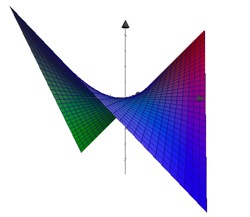
Introductory example: Saddle (surface)
We imagine a three-dimensional coordinate system. Every point \((x_1,y_1)\) on the \(xy\)-plane is associated with the point \((x_1,y_1,z_1)\) where \(z_1=x_1\cdot y_1\).
If \(x\) is fixed, we have an equation of a line: \[z = const. \cdot y\] For example with \(x=2\) we obtain \(z=2\cdot y\). The equations describe straight lines, which run parallel to the \(yz\)-plane.
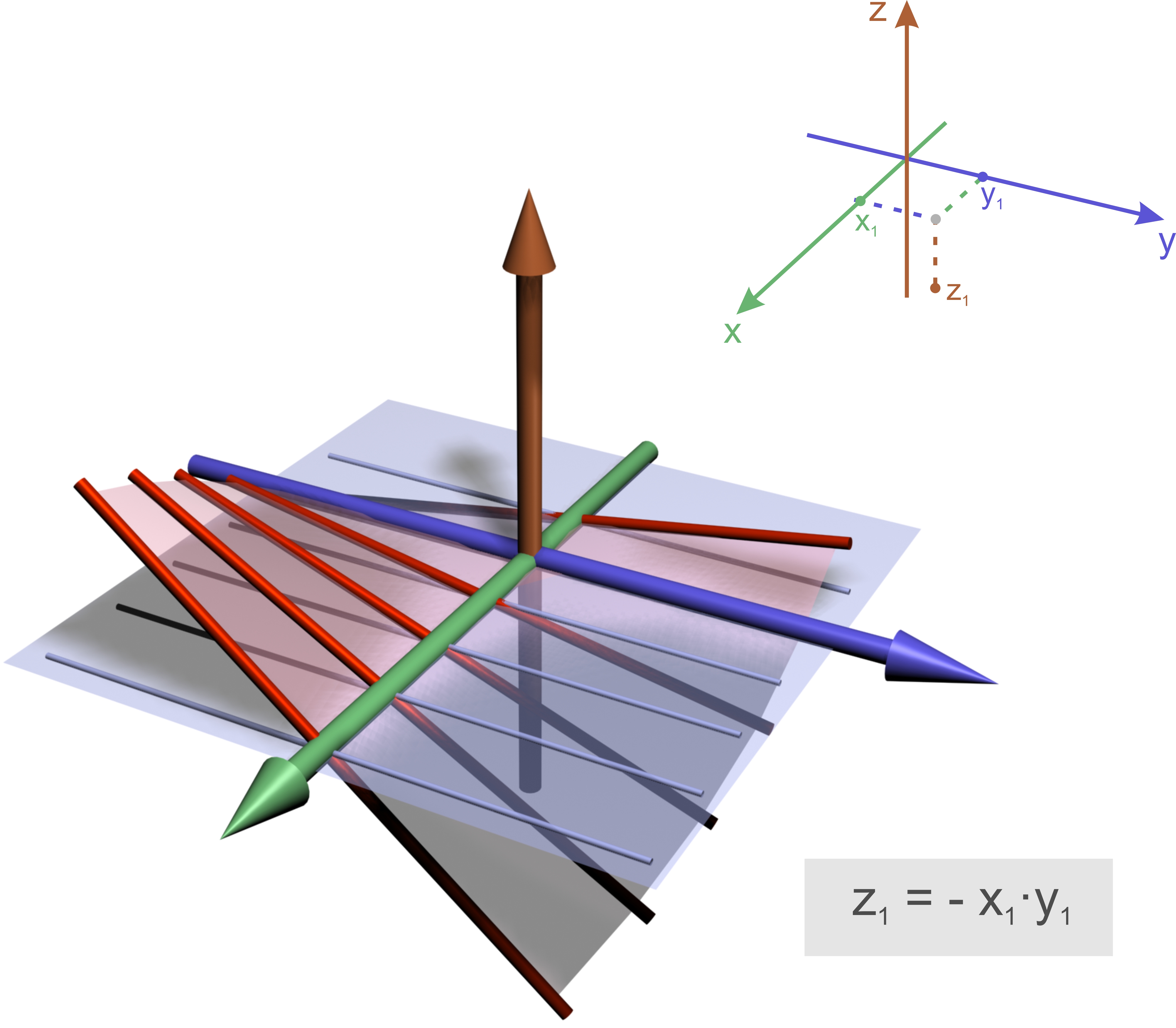
If we vary \(x\) we get a family of straight lines which generates a surface, the so-called saddle (surface).
In general we call every surface generated by the movement of a straight line, a ruled-surface.
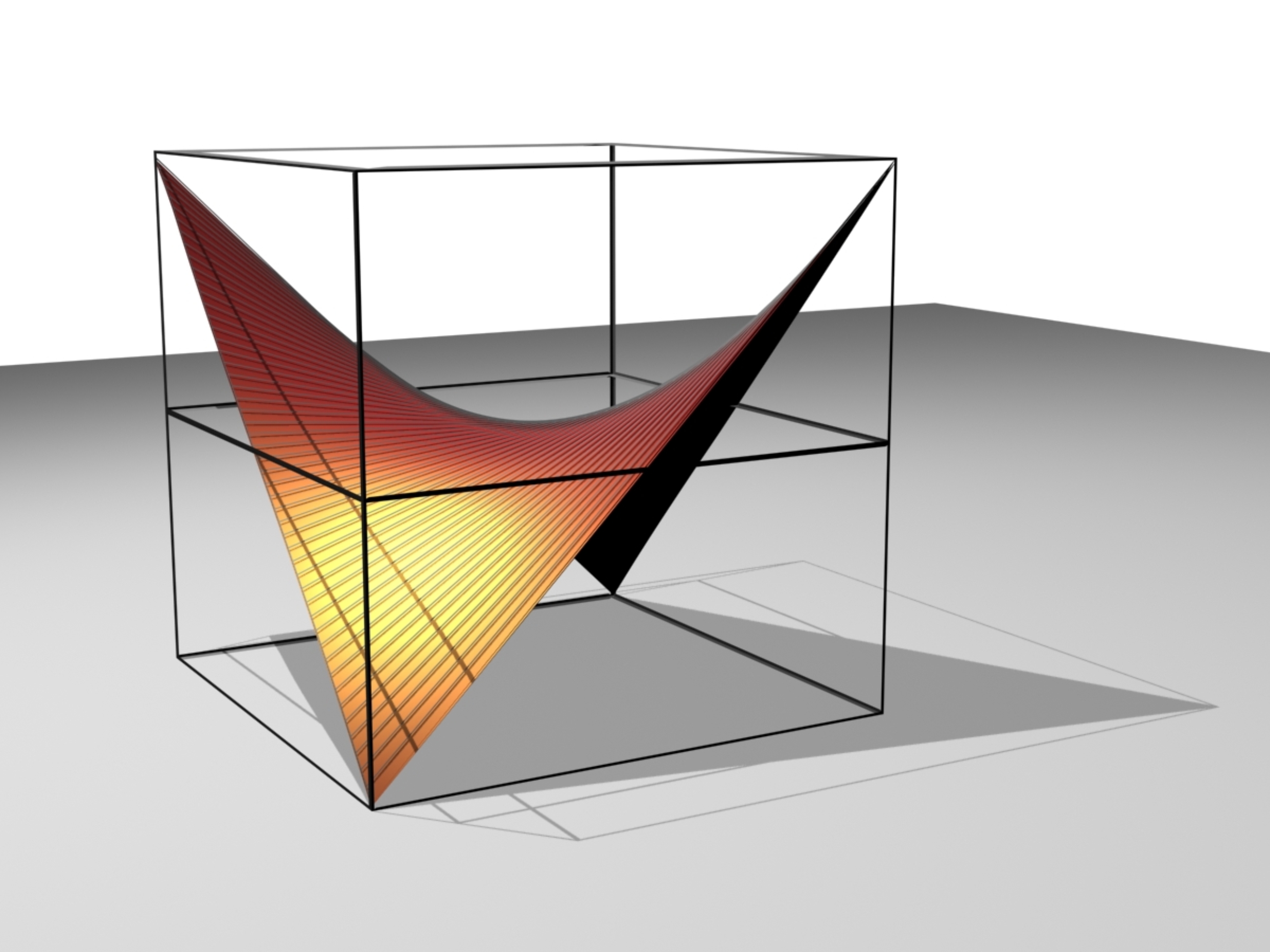
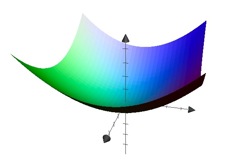
Example: Paraboloid
We consider the function \[f(x,y)=x^2+y^2\]
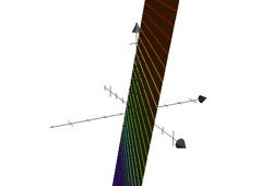
Exercise: Linear functions
We consider the equation \[z(x,y) = 2x + 5y\] Show that the graph of the function is represented by a plane, when you input fixed values of \(x\) (or of \(y\)), e.g. \(x=\{-2, -1, 0, 1, 2\}.\)
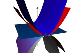
Example: Families of curves
\[f_a(x)=f(a,x)=a\cdot x^2\] In this particular 'function of two variables' the variables are \(x\) and the parameter of the family \(a\). Further example: \(f_a(x) = a\cdot \sin(x)\) is regarded as \(f(a,x) = a\cdot \sin(x)\) or as \(f(x,y) = y\cdot \sin(x)\). The diagram on the right shows the graph of the function \(z=a \cdot x^2\) for \(a=\{-2,...,2\}\).
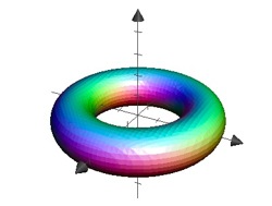
Example: Torus
The equation \[\left(\sqrt{x^2+y^2}-R\right)^2+z^2-r^2=0\] describes a torus. We can picture this as a circle with radius \(r\), which is rotated at a distance \(R\), around the \(z\)-axis. The \(z\)-axis is an axis of symmetry and the \(xy\)-plane a plane of symmetry to the torus.
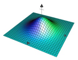
Example: The Bell Curve
The graph of the function \[z=C\cdot e^{-a^2\left(x^2+y^2\right)}\] with constants \(a,C\in \mathbb{R}\) resembles a bell. It is symmetric to the \(z\)-axis.
1.6. Curves and Maps
In this section selected curves are introduced, for example circles and ellipses.
Definition: Curves
A parametrized curve \(K\) is a mapping of the form \[\begin{aligned}K : \left[a, b\right] & \to \mathbb{R}^2 \\ t & \mapsto \left(K_1\left(t \right),K_2\left(t \right)\right) = \left(x(t), y(t) \right),\end{aligned}\] where \(t \in \left[a, b\right]\subset \mathbb{R}\); here \(t\) is called the parameter.
The implicit representation of a curve \(K\) is the zero set of a function \(f\): \[K : \left\{(x,y)\ |\ f(x,y)=0\right\}\]
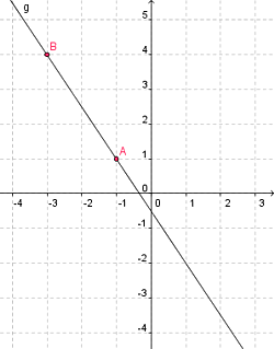
Representing straight lines
The line \(g\) passing through the points \(A = (-1, 1)\) and \(B = (-3, 4)\) has the following parametric representation: \[\left( x = -1 + t(-3 - (-1)), \quad y = \enspace 1 + t(4 - 1) \right)\] and so \[\left(x = -1 - 2t,\quad y = \enspace 1 + 3t\right)\]
Therefore, in general, the parametric representation is: \[\left(x = x_1 + t(x_2 - x_1), \quad y = y_1 + t(y_2 - y_1)\ |\ \forall t\in \mathbb{R}\right)\]
In a more implicit form the line \(g\) is expressed by the equation: \[(4 - 1)(x - (-1)) = (-3 - (-1))(y - 1)\] and so \[3x + 2y + 1 = 0\]
This gives the general form \[(y-y_1) = m\cdot(x-x_1);\] where \(m\in \mathbb{R}\) is the so-called gradient of the straight line. It can be calculated this way \[m = \frac{y_2-y_1}{x_2-x_1}.\]
Representing circles
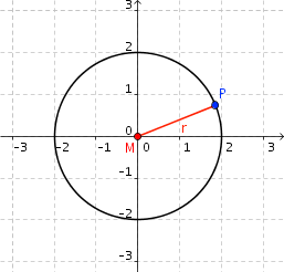
Definition: Circle
A circle is the set of all the points P which have a given distance r from a given point M, thus \[|PM| = r.\] It is fully defined by the point \(M\), its centre, and its radius \(r\).
In a more implicit form the circle around the origin \(M = (0,0)\) with radius \(r=2\) can be written as: \[x^2 + y^2 = 2^2.\]
Alternatively, but equivalently, a circle can also be represented in parametric form: \[(x = 2 \cdot \cos(t),\quad y = 2 \cdot \sin(t)\ |\ 0 \leq t < 2\pi)\]
Representing ellipses
A circle (red) is a special kind of ellipse (blue) (see animation on the right).
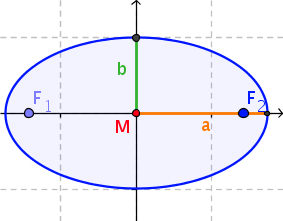
Definition: Ellipse
An ellipse is the set of all points \(P\), whose distances from two given points \(F_1\) and \(F_2\), the so-called foci, sum to a constant. Hence \[|PF_1| + |PF_2| = const.\]
Here you see the so-called string construction of an ellipse. Draw with the mouse on the red spot \(P\) and also change the position of the foci \(F_1\) and \(F_2\) with the orange scroll-bar:
Every point \(P =( x,y )\) of an ellipse with the half-axes \(a\) and \(b\) (see diagram right) satisfies the equation: \[\frac{x^2}{a^2} + \frac{y^2}{b^2} = 1.\] This is the ellipse equation for an ellipse with centre \((0, 0)\) in Cartesian coordinates.
The parametric form equivalent to this is: \[(x = a \cdot \cos(t), y = b \cdot \sin(t)\ |\ 0 \leq t < 2\pi)\]
A further example: Cycloid
If a wheel of radius \(r\) rolls along a level plane (e.g., a car tyre) without slipping and if the movement of a point \(P\) on the edge of the wheel is recorded (e.g., the movement of the valve), then the path of the point P is a so-called cycloid.
We choose, in this case, the distance \(a=|MP|\) from the centre \(M\) of the wheel to the point \(P\) and the so-called angular-displacement \(t\) as our parameters (see adjacent applet). The parametric representation of the curve is then: \[(x = r\cdot t - a \cdot \sin(t), y = r - a \cdot \cos(t))\]
Depending on the position of the point \(P\) we get different types of cycloid. If \(a=r\) the curve is called a common cycloid, if \(a>r\) a prolate cycloid and if \(a\lt r\) a curtate cycloid.

1.7. Exercises
Tasks for Chapter 1 "Functions"
Task 1: Parabolas I
The graphs of the functions \(f\), \(g\) with \(f(x) = ax^2+ bx + c\) and \(g(x) = d(x-e)^2+ h\) should show the samme parabola. What is the relationship between the variables \(a\), \(b\), \(c\), \(d\), \(e\) and \(h\)?
Task 2: Parabolas II
We consider the parables \(\P_b) with the equation \(f(x) = 2x^2+ bx + 1\), \(b \in \mathbb{R}\).
- Determine the vertex \(S_b\) of the parabolas \(P_b\) (thus depending on \(b\)).
- Draw - for example with the help of the program GeoGebra (downloadable free of charge from http://www.geogebra.at) the locus line \(OS_b\) on which the vertex of \(P_b\) moves when \(b\) is varied. A screenshot of this task should be included in the solution of the task.
- Determine the equation for the locus line \(OS\).
Task 3: Exponential function
- Compare the two functions with \(y = a \cdot 2^x\) and \(y = 2^{(x+d)}\) for different values \(a,d \in \mathbb{R}\). For which \(a\) or \(d\)-values do the graphs of the two functions match?
- The general exponential function can be calculated with the equation \(f(x) = a \cdot b^{cx+d}\) with \(a,c,d \in \mathbb{R}; b \in \mathbb{R}^+\). This equation is equivalent to an equation with only three parameters \(A,B,C\) where \(A,B,C \in \mathbb{R}\) or \(\mathbb{R}^+\). Give the relationship between \(A,B, C\) and \(a,b,c,d\).
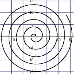
Task 4: Spiral
Draw the curve \(K(t) = (t \cdot \cos(t), t \cdot \sin(t))\) for \(0 < t < 20\). The curve can be thought of as resulting from a movement and dynamically interpreted, if \(t\) is understood as time. This curve is called a spiral.
- Describe this movement!
- Specify the equation of the shown spiral!
Task 5: Ellipse
Given is an ellipse \(E(x,y): \frac{x^2}{a^2} + \frac{y^2}{b^2} = 1\); \(a,b \in \mathbb{R}^+\). Specify the equation of the tangent to the ellipse in the ellipse point \(P(x_0,y_0)\).
Note: Start from the circle \(K_a: x^2+ y^2= a^2\) and create \(E\) by stretching or compressing \(K_a\) by the factor \(\frac{b}{a}\) parallel to the \(y\)-axis. Then start from a circle tangent.
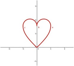
Task 6: The heart
There are different possibilities how to draw a heart using mathematical functions. In particular a heart can have many different forms. Using function pieces (in GeoGebra) draw a heart shape. The image on the right shows one example of how it can be achieved.
Task 7: Function of two variables
- Describe the graph \(G\) of the function \(f(x,y) = x^2+ y^2\) by cutting \(G\) with selected planes and describing the resulting figures.
- Consider the two planes \(f(x,y) = 4x + y + 3\) and \(g(x,y) = -x + 3y - 5\) in a joint coordinate system. Show that these two planes are perpendicular to each other.
2. Outlook: Content of the Course
- 1. Functions
-
1.1. Linear and Quadratic Functions
-
1.2. Power Functions, Polynomials and Power Series
-
1.3. The Exponential Function and Growth
-
1.4. Trigonometric Functions
-
1.5. Multivariable Functions
-
1.6. Curves and Maps
-
1.7. Exercises
-
-
2. Equations
-
2.1. Basic Concepts and Solving Methods
-
2.2. Linear and Quadratic Equations
-
2.3. Trigonometric Equations
-
2.4. Exponential and Logarithmic Equations
-
2.5. Complex numbers
-
2.6. Exercises
-
-
3. Sequences and Limits
-
3.1. Introduction to sequences
-
3.2. Different ways of defining a sequence
-
3.3. Important examples of sequences
-
3.4. Basic properties of sequences
-
3.5. Limit of a function
-
3.6. Operations with limits
-
3.7. Continuity of a function
-
3.8. Properties of continuous functions
-
3.9. Exercises
-
-
4. Differentiation
-
4.1. Derivative
-
4.2. Properties of derivative
-
4.3. Derivatives of Trigonometric Functions
-
4.4. The Chain Rule
-
4.5. The Exponential Function and the Logarithm
-
4.6. Extremal Value Problems
-
4.7. Exercices
-
-
5. Integration
-
5.1. The Concept
-
5.2. Fundamental theorem of calculus
-
5.3. Integrals of elementary functions
-
5.4. Integration techniques
-
5.5. Applications
-
5.6. Exercises
-
-
6. Differential Equations
-
6.1. Differential Equation
-
6.2. Solving a 1st order ODE
-
6.3. 2nd and higher order ODEs
-
6.4. Exercises
-