Lecture - Fundamental Concepts
4. Receiver Response
4.3. Sampling, weighting, gridding
Sampling
As previously mentioned, the visibilities are only measured at discrete locations ") . Therefore, the measured visibilities are given by the multiplication of the true visibility function
. Therefore, the measured visibilities are given by the multiplication of the true visibility function  and a sampling function
  . Hence, the dirty image
  is then given by the convolution of their Fourier transforms:
![\displaystyle B^\text{D} = \mathcal{FT}[V^\text{S}] = \mathcal{FT}[V \cdot S] = \mathcal{FT}[V] \star \star \mathcal{FT}[S] \text{,}](https://wuecampus.uni-wuerzburg.de/moodle/filter/tex/pix.php/ae19d1b8e17a3ebbdd115e1eeff5e233.gif "\displaystyle B^\text{D} = \mathcal{FT}[V^\text{S}] = \mathcal{FT}[V \cdot S] = \mathcal{FT}[V] \star \star \mathcal{FT}[S] \text{,}")
in which ![\mathcal{FT}[x]](https://wuecampus.uni-wuerzburg.de/moodle/filter/tex/pix.php/290d52c31264c1e54193648e665e8ad5.gif "\mathcal{FT}[x]") denotes the Fourier transform of
denotes the Fourier transform of  and the double-star
  indicates a two-dimensional convolution.
Weighting
Furthermore, as also previously mentioned, the visibilities can be weighted by multiplying a weighting function  to the visibilities
  :
:

This weighting function consists of three individual factors:
 accounts for different telescope properties within an array (e.g. different
  ,
,  ,
,  and
and  ),
), is a taper that controls the beam shape,
 weights the density of the measured visibilities.
The -factor affects the angular resolution and sensitivity of the array. On the one hand side, the highest angular resolution can be achieved by weighting the visibilities as if they had been measured uniformly over the entire ") -plane. Therefore, this weighting scheme is called uniform weighting. Since the density of the measured visibilities is higher at the center of the -plane, the visibilities in the outer part are over-weighted leading to the highest angular resolution. On the other hand, the highest sensitivity is achieved if all measured visibilities are weighted by identical weights. This weighting scheme is called natural weighting. The main properties of both schemes are summarized in the following:
-plane. Therefore, this weighting scheme is called uniform weighting. Since the density of the measured visibilities is higher at the center of the -plane, the visibilities in the outer part are over-weighted leading to the highest angular resolution. On the other hand, the highest sensitivity is achieved if all measured visibilities are weighted by identical weights. This weighting scheme is called natural weighting. The main properties of both schemes are summarized in the following:
- natural weighting:

- broader synthesized beam
- highest sensitivity
- uniform weighting:
}") , in which
, in which ") is the number of visibilities occurring within an area of constant size around the weighted visibility
is the number of visibilities occurring within an area of constant size around the weighted visibility- highest resolution
- lowest sensitivity
With this weighting function , the dirty image is given by
![\displaystyle B^\text{D} = \mathcal{FT}[V^\text{W}] = \mathcal{FT}[W \cdot V^\text{S}] = \mathcal{FT}[W] \star \star \mathcal{FT}[V^\text{S}] = \mathcal{FT}[W] \star \star (\mathcal{FT}[V] \star \star \mathcal{FT}[S]) \text{.}](https://wuecampus.uni-wuerzburg.de/moodle/filter/tex/pix.php/2eca0fb08d98b8eadba80a378194ca7b.gif "\displaystyle B^\text{D} = \mathcal{FT}[V^\text{W}] = \mathcal{FT}[W \cdot V^\text{S}] = \mathcal{FT}[W] \star \star \mathcal{FT}[V^\text{S}] = \mathcal{FT}[W] \star \star (\mathcal{FT}[V] \star \star \mathcal{FT}[S]) \text{.}")
Gridding
To use the time advantage of the fast Fourier transform (FFT) algorithm, the visibilities must be interpolated onto a regular grid of size ") , resulting in an image of size
, resulting in an image of size  . This interpolation, also called gridding, is done at first by convolving the weighted discrete visibility
  with an appropriate function
  to obtain a continuous visibility distribution. This continuous visibility distribution is then resampled at points of the regular grid with spacings
  and
and  by multiplying a two-dimensional Shah-function
  , given by
 |
|---|
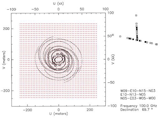
Fig. 2.32 Illustration of the gridding process. The real -tracks measured by the IRAM interferometer at Plateau de Bure in France (black dots) have to be interpolated onto a regular grid of  pixels (red dots). Taken from: U. Klein pixels (red dots). Taken from: U. Klein |
 = \sum_{\text{j} = -\infty}^{\infty} \sum_{\text{k} = -\infty}^{\infty} \delta^2\left(j-\frac{u}{\Delta u}, k-\frac{v}{\Delta v}\right) \text{.}")
After these modifications, the visibility  is given by
 ![\displaystyle V^\text{G} = G \cdot (C \star \star V^\text{W}) = G \cdot [C \star \star (W \cdot V^\text{S})] = G \cdot [C \star \star (W \cdot V \cdot S)]](https://wuecampus.uni-wuerzburg.de/moodle/filter/tex/pix.php/24e98dae931507ec8c75522931b13c87.gif "\displaystyle V^\text{G} = G \cdot (C \star \star V^\text{W}) = G \cdot [C \star \star (W \cdot V^\text{S})] = G \cdot [C \star \star (W \cdot V \cdot S)]")
and the dirty image  reads
reads![\displaystyle \tilde{B^\text{D}} = \mathcal{FT}[G] \star \star (\mathcal{FT}[C] \cdot \mathcal{FT}[V^\text{W}]) = \mathcal{FT}[G] \star \star \{ \mathcal{FT}[C] \cdot [\mathcal{FT}[W] \star \star (\mathcal{FT}[V] \star \star \mathcal{FT}[S])]\} \text{.}](https://wuecampus.uni-wuerzburg.de/moodle/filter/tex/pix.php/1b44c8e537f9f7143cf62d73d416bec3.gif "\displaystyle \tilde{B^\text{D}} = \mathcal{FT}[G] \star \star (\mathcal{FT}[C] \cdot \mathcal{FT}[V^\text{W}]) = \mathcal{FT}[G] \star \star \{ \mathcal{FT}[C] \cdot [\mathcal{FT}[W] \star \star (\mathcal{FT}[V] \star \star \mathcal{FT}[S])]\} \text{.}")
This gridding process is illustrated in the Fig. 2.29, in which real -tracks measured by the IRAM interferometer at Plateau de Bure in France are shown as black dotted ellipses. Furthermore, a regular grid, onto which the visibilities have been interpolated, is shown as red dots.
Since the sampling intervals and in the -plane are inversely proportional to the sampling intervals  and
and  in the image plane (
  and
and  for a grid of size
  ), the maximum map size in one domain is given by the minimum sampling interval in the other. Therefore, it is important to choose appropriate sampling intervals and . If and are chosen to be too large for example, this will result in artefacts in the image plane produced by reflections of structures from the map edges, which is called aliasing.
The most effective way to deal with this aliasing is to use a convolution function for which the Fourier transform in the image plane ![\mathcal{FT}[C]](https://wuecampus.uni-wuerzburg.de/moodle/filter/tex/pix.php/7265b9d7b7857f89d7fdad5bc301eb5a.gif "\mathcal{FT}[C]") decreases rapidly at the image edges and is nearly constant over the image. Therefore, the simplest choice for the convolution function is a rectangular function, but with this choice the aliasing would be strongest. A better choice would be a sinc function, however a Gaussian-sinc function (product of a Gaussian and a sinc function) leads to the best suppression of aliasing.
decreases rapidly at the image edges and is nearly constant over the image. Therefore, the simplest choice for the convolution function is a rectangular function, but with this choice the aliasing would be strongest. A better choice would be a sinc function, however a Gaussian-sinc function (product of a Gaussian and a sinc function) leads to the best suppression of aliasing.
Finally, the gridding modifications must be corrected after the Fourier transform by dividing the dirty image ") by the inverse Fourier transform of the gridding convolution function
by the inverse Fourier transform of the gridding convolution function ") . Therefore, the so-called grid-corrected image
. Therefore, the so-called grid-corrected image ") is given by
is given by} \text{.}](https://wuecampus.uni-wuerzburg.de/moodle/filter/tex/pix.php/38a39a2ff58598a9e9090adcf122a3df.gif "\displaystyle \tilde{B^\text{D}_\text{C}}(\xi_\text{m},\eta_\text{m}) = \frac{\tilde{B^\text{D}}(\xi_\text{m},\eta_\text{m})}{\mathcal{FT}[C](u,v)} \text{.}")