Demokurs: Introduction to Engineering Mathematics
1. Functions
1.6. Curves and Maps

In this section selected curves are introduced, for example circles and ellipses.

Definition: Curves
A parametrized curve \(K\) is a mapping of the form \[\begin{aligned}K : \left[a, b\right] & \to \mathbb{R}^2 \\ t & \mapsto \left(K_1\left(t \right),K_2\left(t \right)\right) = \left(x(t), y(t) \right),\end{aligned}\] where \(t \in \left[a, b\right]\subset \mathbb{R}\); here \(t\) is called the parameter.
The implicit representation of a curve \(K\) is the zero set of a function \(f\): \[K : \left\{(x,y)\ |\ f(x,y)=0\right\}\]
Representing straight lines
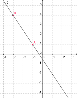
The line \(g\) passing through the points \(A = (-1, 1)\) and \(B = (-3, 4)\) has the following parametric representation: \[\left( x = -1 + t(-3 - (-1)), \quad y = \enspace 1 + t(4 - 1) \right)\] and so \[\left(x = -1 - 2t,\quad y = \enspace 1 + 3t\right)\]
Therefore, in general, the parametric representation is: \[\left(x = x_1 + t(x_2 - x_1), \quad y = y_1 + t(y_2 - y_1)\ |\ \forall t\in \mathbb{R}\right)\]
In a more implicit form the line \(g\) is expressed by the equation: \[(4 - 1)(x - (-1)) = (-3 - (-1))(y - 1)\] and so \[3x + 2y + 1 = 0\]
This gives the general form \[(y-y_1) = m\cdot(x-x_1);\] where \(m\in \mathbb{R}\) is the so-called gradient of the straight line. It can be calculated this way \[m = \frac{y_2-y_1}{x_2-x_1}.\]
Representing circles
Definition: Circle
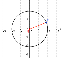
A circle is the set of all the points P which have a given distance r from a given point M, thus \[|PM| = r.\] It is fully defined by the point \(M\), its centre, and its radius \(r\).
In a more implicit form the circle around the origin \(M = (0,0)\) with radius \(r=2\) can be written as: \[x^2 + y^2 = 2^2.\]
Alternatively, but equivalently, a circle can also be represented in parametric form: \[(x = 2 \cdot \cos(t),\quad y = 2 \cdot \sin(t)\ |\ 0 \leq t < 2\pi)\]
Representing ellipses
A circle (red) is a special kind of ellipse (blue) (see animation on the right).
Definition: Ellipse
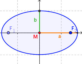
An ellipse is the set of all points \(P\), whose distances from two given points \(F_1\) and \(F_2\), the so-called foci, sum to a constant. Hence \[|PF_1| + |PF_2| = const.\]
Here you see the so-called string construction of an ellipse. Draw with the mouse on the red spot \(P\) and also change the position of the foci \(F_1\) and \(F_2\) with the orange scroll-bar:
Every point \(P =( x,y )\) of an ellipse with the half-axes \(a\) and \(b\) (see diagram right) satisfies the equation: \[\frac{x^2}{a^2} + \frac{y^2}{b^2} = 1.\] This is the ellipse equation for an ellipse with centre \((0, 0)\) in Cartesian coordinates.
The parametric form equivalent to this is: \[(x = a \cdot \cos(t), y = b \cdot \sin(t)\ |\ 0 \leq t < 2\pi)\]
A further example: Cycloid
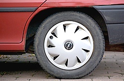
If a wheel of radius \(r\) rolls along a level plane (e.g., a car tyre) without slipping and if the movement of a point \(P\) on the edge of the wheel is recorded (e.g., the movement of the valve), then the path of the point P is a so-called cycloid.
We choose, in this case, the distance \(a=|MP|\) from the centre \(M\) of the wheel to the point \(P\) and the so-called angular-displacement \(t\) as our parameters (see adjacent applet). The parametric representation of the curve is then: \[(x = r\cdot t - a \cdot \sin(t), y = r - a \cdot \cos(t))\]
Depending on the position of the point \(P\) we get different types of cycloid. If \(a=r\) the curve is called a common cycloid, if \(a>r\) a prolate cycloid and if \(a\lt r\) a curtate cycloid.