Demokurs: Introduction to Engineering Mathematics
1. Functions
1.3. The Exponential Function and Growth

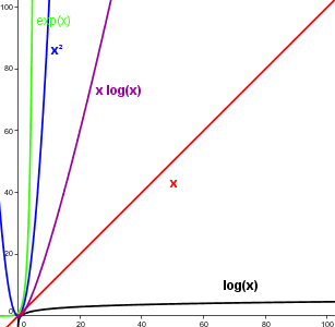
In this chapter we meet a particularly important function: the exponential function. Afterwards we categorize the growth of arbitrary functions with the help of the growth of functions we already know.
Introductory example: Linear and exponential growth
Example 1: Growth of capital with simple interest
When using simple interest, the amount of interest added each year to the initial capital (or principal) \(K_0\), is \(K_0\cdot\frac{p}{100}\). The interest in following years is calculated only on \(K_0\). We can therefore assume that the yearly interest is withdrawn by the investor. It can be deduced that the capital after \(n\) years is \[K(n) = K_0 + K_0\cdot\frac{p}{100}\cdot n\]
When using compound interest the interest is paid out on the interest of the preceding years, i.e., the initial capital \(K_0\) is multiplied every year by \((1+\frac{p}{100}).\) It can be deduced that the capital after \(n\) years is \[K(n) = K_0\cdot(1+\frac{p}{100})^n\]
Exercise.
Explain how this formula was derived!
Both formulae for the growth of the capital are valid only for complete years (\(n\in\mathbb{N}\)), as the bank pays interest annually. The graph of the capital is therefore a discrete graph.
By approximation we can also work with the exponent \(x\in\mathbb{R}\), in order to calculate the capital at arbitrary times (e.g., \(x=1.75\) years). The graph of the capital after an arbitrary time period \(x\) is a continuous curve. (This continuous expansion can be switched on and off in the applet to the right using the tick box.)
The growth of capital governed by the functional equation \(K(x) = K_0\cdot(1+\frac{p}{100})^x\) is called exponential growth. Here the independent variable \(x\) is the exponent and this new type of function is therefore called an exponential function.

The general exponential function
Definition 1: Exponential function to the base \(a\)
The function \[f: \mathbb{R}\rightarrow\mathbb{R}, f(x) = a^x = \exp(x\cdot\log(a)) \qquad (a\in\mathbb{R}^+, a\neq 1)\] is called the exponential function to the base \(a\).
Theorem 1: Functional equation
For all \(x,y\in\mathbb{R}\) we have: \[a^{(x+y)}=a^x\cdot a^y\]
Proof. The functional equation follows directly from the theorem of multiplication of two powers with the same basis: \[b^m\cdot b^n = b^{m+n}\]
\(\square\)
Properties of a general exponential function \(x\mapsto a^x\)
-
The exponential function is defined for all \(x\in\mathbb{R}.\)
-
It has only positive output.
-
All exponential functions of the form \(f(x) = a^x\) pass through the point (0,1).
-
For \(0 \lt a \lt 1\) the function \(f(x)\) is monotonically decreasing, for \(a=1\) it is constant and for \(a>1\) monotonically increasing.
-
The graphs of \(f(x) = a^x\) and \(g(x) = a^{-x} = \frac{1}{a^x}\) are symmetric about the \(y\)-axis. For both graphs the \(x\)-axis is a horizontal asymptote.
-
For \(0 < a < 1\) the function \(f(x) = a^x\) is monotonically decreasing, \(f\) diverges for \(x \rightarrow -\infty\) and converges to \(0\) for \(x \rightarrow \infty\).
-
For \(a=1\) \(f\) is constant
-
For \(a > 1\) the function \(f(x) = a^x\) is monotonically increasing. \(f\) diverges for \(x \rightarrow \infty\) and converges to \(0\) for \(x \rightarrow -\infty\).
Interactivity. Explore the behaviour of the exponential function under varying parameters using the Geogebra app.
-
(Exercise on \(x \mapsto a^x\)) Set \(m\) and \(b\) to 1, \(c\) and \(d\) to 0 and vary the value of the base \(a\) using the scrollbar. Describe how the graph changes for different values of \(a\). Verify the properties of the function \(x \mapsto a^x\) given above.
-
Why doesn't the function \(f(x)\) exist for negative \(a\)?
-
(Exercise on \(x\mapsto m\cdot a^x\)) Let \(a\) again be fixed (and non-zero). Describe the effect on the graph by varying \(m\) and find a certain characteristic for certain pairs of numbers.
-
(Exercise on \(x\mapsto a^{b\cdot x}\)) From now on let \(a\) be fixed (and non-zero). Describe the effect on the graph by varying \(b\) and find a certain characteristic for certain pairs of numbers.
-
(Exercise on \(x\mapsto a^x+c\)) Again set \(m\) and \(b\) to 1 and \(d\) to 0 and vary the value of \(c\) using the scroll bar. Describe how the graph changes.
-
(Exercise on \(x\mapsto a^{x+d}\)) Again set the value of \(m\) and \(b\) to 1 and \(c\) to 0 and vary the value of \(d\) using the scroll bar. Describe how the graph changes.
The logarithm - the inverse of the exponential function
The inverse of the exponential function is the logarithm \[\log_a(x): \mathbb{R}^+\rightarrow\mathbb{R}.\] It is continuous and strictly monotonous increasing.
The logarithm function results as the inverse function by rearranging the exponential function: \[y=f(x)=a^x\] Then \[x=f^{-1}(y)=log_a(y)\] To plot the function in the familiar coordinate system the form \(x \rightarrow f^{-1}(x)\) is most commonly used.
Interactivity. Work through the following assignments using the Geogebra app.
-
Vary the value of \(a\) using the scroll bar and describe how the graph changes for different values of \(a\). What do all the functions have in common? What differences are there for different values of \(a\)?
-
What do you notice if you compare the exponential and the logarithmic functions? Describe the position of both graphs in relation to one another.
Theorem 2 (Functional equation)
For all \(x,y\in\mathbb{R}^+\) we have: \[\log_a(x\cdot y)=\log_a(x)+\log_a(y)\]
Proof.
The functional equation follows directly from the functional equation of the exponential function (theorem 1): \[\log_a(x\cdot y) = \log_a(a^{\xi}\cdot a^{\eta}) =\] \[= \log_a(a^{\xi+\eta}) = \xi+\eta = \log_a(x)+\log_a(y)\]
\(\square\)
New terms:
-
Exponential growth
-
Exponential function
-
Logarithm