Demokurs: Introduction to Engineering Mathematics
1. Functions
1.1. Linear and Quadratic Functions

This chapter contains the definition of the term function and examines linear and quadratic functions.

What is a function?
Example 1.
The following relationship exists between the speed of sound in metres per second, \(c\), and the air temperature in degrees Celsius, \(\theta\): \[c=331,5\cdot\sqrt{1+\frac{\theta}{273}} \qquad \text{for } \theta>-273\] \(c=c(\theta)\) is a function of \(\theta\).
Definition 1: Function
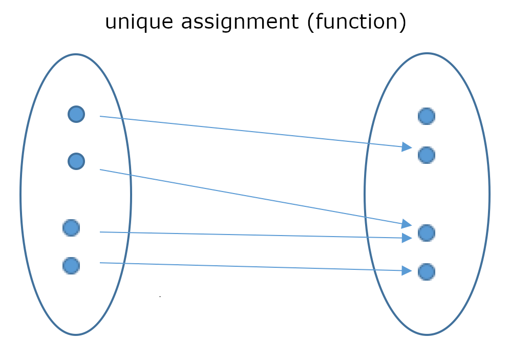
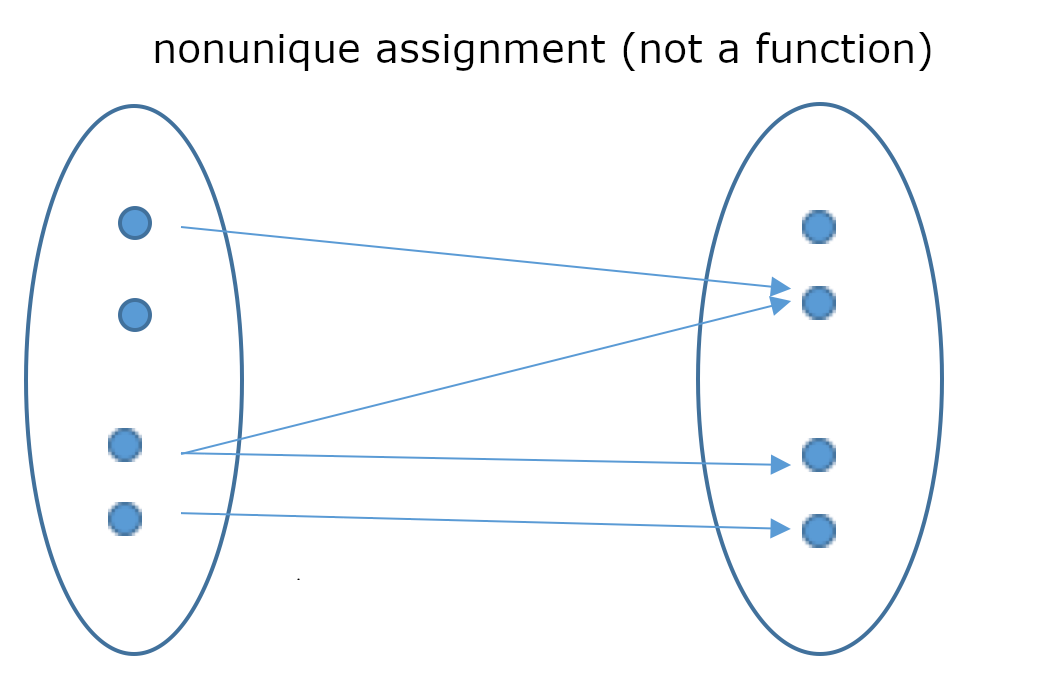
For arbitrary sets \(A\) and \(B\), a function (or map) \(f: A\rightarrow B\) is a rule which assigns a unique value \(y=f(x) \in B\) to \(x \in A\). Here \(A\) is called domain and \(B\) the codomain. The graph of \(f\) is the set \(G_f = \{(x,y) \in A\times B : y=f(x)\}.\)
Explanation: This means that a function is a unique assignment rule.
This example, assigns to each natural number \(x\) its square \(y=f(x)=x^2\):
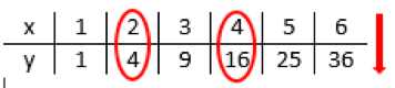
Usually, the functions that are relevant within this course are represented (plotted) as a graph in a coordinate system. A graph is – as defined above – a set of points, which results in the common curve depiction. Those points have the shape \((x|f(x))\).
Linear functions
The functional equation of a linear function \(f:x\in\mathbb{R}\mapsto f(x)\in\mathbb{R}\) can be written as: \[f(x) = m\cdot x + t, \qquad m,t\in\mathbb{R}\]
Here, \(m\) is called the slope or gradient and \(t\) the \(y\)-intercept of the function (more precisely: of the graph of the function).
For a positive slope/ gradient \(m>0\) the line increases (rises), for a negative slope/ gradient \(m<0\) the line decreases (falls). The larger the absolute value of \(m\), the steeper the line rises or falls: The larger a positive gradient is, the steeper the line increases; the smaller a negative gradient is, the steeper the line decreases.
\(m=0\) results in the special case of a line which is parallel to the \(x\)-axis, that is, horizontal: \[f(x)=t\]
One should note that lines parallel to the \(y\)-axis cannot be depicted by linear functions, because the slope would have to be infinitely large. In that case infinitely many values would have to be assigned to one x-value (which would contradict the definition of a function).
Such linear functions can be represented with the following equation (which is not a function!): \[x=a, a\in\mathbb{R}\]As \(t\) increases or decreases the value of the function independently from \(x\) (this means \(t\) does not change for different \(x\) values/ is the same for all \(x\)), we can move the whole graph along the \(y\)-axis. For positive \(t\) the graph moves up and for negative \(t\) it moves down. If \(t=0\), then the line passes through the origin; in this case we have \(f(0)=m∙0+t=t=0\).
Interactivity. Explore the influence of the parameters \(m\) and \(t\) on the linear function.
This notation means that the function rule \(f\) assigns to each value \(x\) (the „pre-image“) a function value \(f(x)\) (the „image“). Both \(x\) and \(f(x)\) lie in \(\mathbb{R}\) in this case.
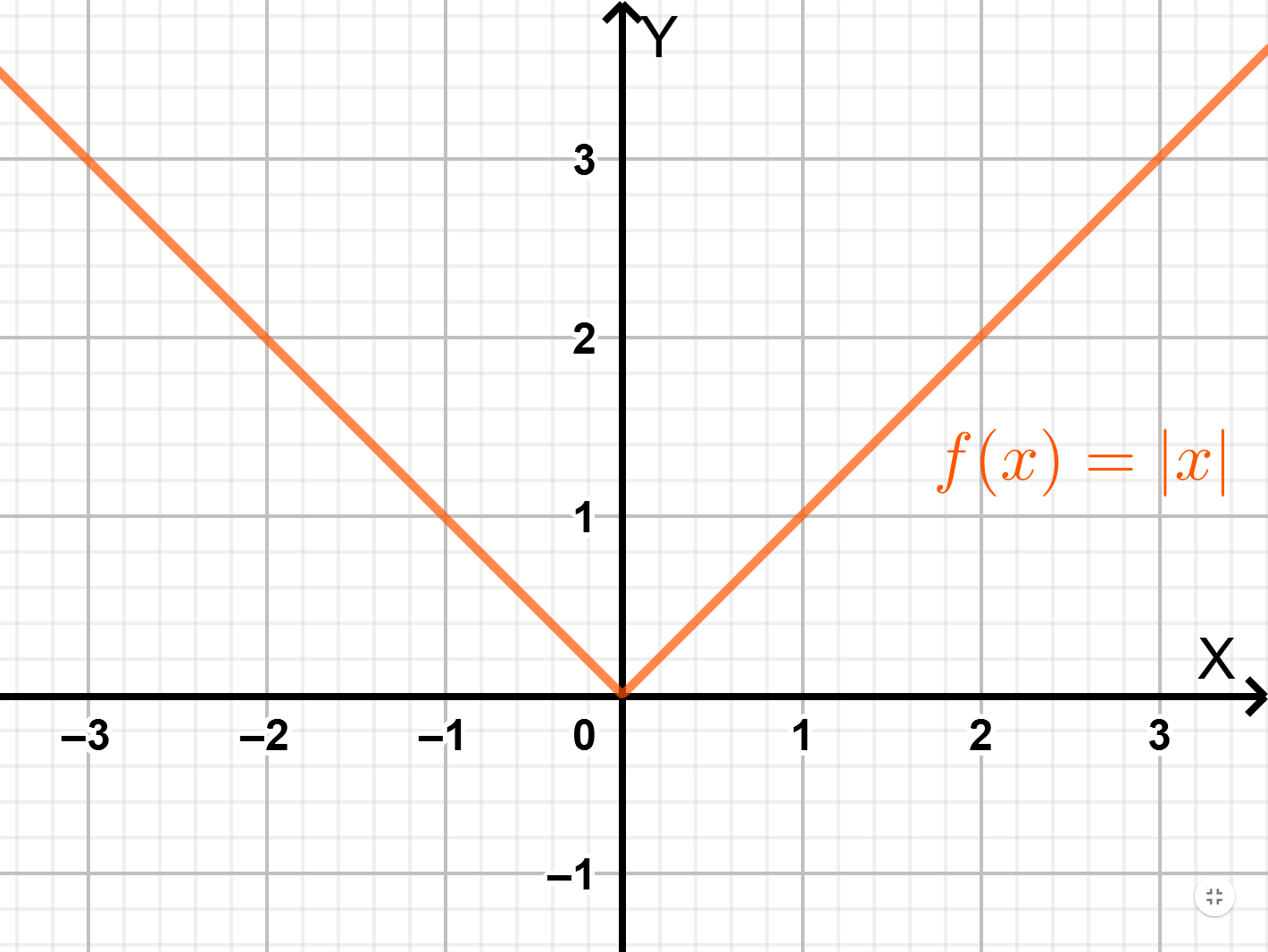
The absolute value \(|a|\) of a number \(a\) is its value without the sign: \[|3|=3\] \[|-3|=3\]
Acccordingly, one can define the absolute value function: \[f(x)=|x|=\begin{cases} x, \text{for } x\geq 0\\ -x, \text{for } x < 0\end{cases}\]
Calculating the gradient and the \(y\)-intercept
The gradient of a linear function is calculated using the so-called 'gradient triangle' as follows: \[m=\frac{\Delta y}{\Delta x} = \frac{\Delta f(x)}{\Delta x} = \frac{f(x_2)-f(x_1)}{x_2-x_1}\]
Here, the vertical distance between two points on the graph is divided by the horizontal distance of those two points (to be more precise, the values of the distances). So, the gradient depicts how the vertical value changes when the horizontal value changes.
As an example, road gradients are measured in a similar way. Here, the difference in altitude covered by the car is measured while it moves 100m in the vertical direction. (So, the actual distance is the hypotenuse of the resulting right-angle triangle) With this in mind - \(x\) as the difference in altitude per 100m - the gradient is expressed as a percentage.

The \(y\)-intercept \(t\) equals the value the function has for \(x=0\), which is calculated by evaluating the function for \(0\): \[t = f(0)\]
Plotting the graph of the function
To plot the graph of the function you should memorize the following steps:
-
Starting at the origin move along the \(y\)-axis until you reach \(t\). We call this point \(P\).
-
Starting at \(P\) move up, vertically, the value of the numerator of \(m\) and move right, horizontally, the value of the denominator of m. We call this point \(Q\).
-
The graph is a straight line through \(P\) and \(Q\).
If \(m\) has already been calculated, \(m\) can be used as the numerator, and \(1\) as the denominator, since \(m=\frac{m}{1}\)
Calculating the angle \(\alpha\) between the straight line and the \(x\)-axis
With the definition for the trigonometric function of the tangent in right-angled triangles ((the length of) the opposite side divided by (the length of) the adjacent side) it is true that: \[tan(\alpha ) = \frac{\Delta f(x)}{\Delta x} = m\]
according to the definition of the gradient m and therefore: \[\alpha = arctan(m)\]
Zeroes
A linear function has exactly one zero (\(f(x) = 0\)), that means there is only one intersection with the \(x\)-axis. The exception being the case where \(m=0\). Here \(f\) is a constant function and thus the graph is a line parallel to the \(x\)-axis: \(f(x) = t\). Such a function does not have a zero for \(t\neq 0\). For \(t=0\) it holds: \(f(x)=0\). In this case the function has infinitely many zeros.
To calculate the zero \(x_0\) set \(f(x_0)=m\cdot x_0+t = 0\) and solve the equation for \(x_0\): \[x_0 = -\frac{t}{m}\]
Relationships between graphs of linear functions
Two lines \(G_f\) and \(G_g\) are parallel if, and only, if their gradients \(m_1\) and \(m_2\) are equal: \[m_1 = m_2 \Leftrightarrow G_f \parallel G_g\]
So, parallel lines \(f_1, f_2, f_3,\ldots \) only differ through their \(y\)-intercepts \(t_1, t_2, t_3,\ldots \) This means the functions emanate from each other through translations (parallel shifts) in the vertical direction (upwards and downwards).
Two lines \(G_f\) and \(G_g\) are perpendicular, if and only if, the product of their gradients \(m_1\) and \(m_2\) equals -1: \[m_1\cdot m_2 = -1 \Leftrightarrow G_f \perp G_g\]

Exercise.
Justify this relationship between \(m_1\) and \(m_2\).
Quadratic functions
The general form of the quadratic function \(f:x\mapsto f(x)\) is: \[f(x) = a\cdot x^2 + b\cdot x + c, \qquad a \neq 0,b,c\in\mathbb{R}\]
Graphs of quadratic functions are parabolas.
The coefficient of \(x^2\) i.e. a, determines the form of the parabola. If \(a\) is a positive number, the parabola opens upwards; if negative, it opens downwards. The bigger the value of \(|a|\) is chosen, the graph appears more closed. Conversely the shape of the parabola becomes less closed for a smaller value of \(|a|\).
A change in the parameter \(c\) shifts the parabola in the \(y\)-direction, because \(c\) is independent from \(x\). As a result changes in \(x\) have no influence on \(c\). If \(c\) is increased by one, the graph is displaced upwards by one. On the other hand if \(c\) is decreased by one, the graph is displaced downwards by one.
\(c\) is therefore basically the \(y\)-intercept which we encountered by looking at straight lines.
\(|a|\) denotes the absolute value of \(a\), that is the value of \(a\) "without the sign".
Identifying vertices
The vertex of the parabola is either the absolute minimum point (if \(a\) is a positive number) or the absolute maximum point (if \(a\) is a negative number). If the function is converted to the vertex form below by completing the square and using the binomial formula, the coordinates of the vertex can be read off directly: \[f(x) = a\cdot (x-x_s)^2 + y_s.\]
With this form of the equation the graph of \(f\) can be seen as a variation of the (standardized) parabola with the form \(g(x)=x^2\). \(f\) generates from this by shifting it to the right by \(x_S\), up by \(y_S\) and by dilation/compression by the factor \(a\).
From the general form of the quadratic equation (see above), we get the coordinates of the vertex as: \[x_s = -\frac{b}{2a}\] \[y_s = \frac{4ac-b^2}{4a}\]
The vertex then has the coordinates \((x_s, y_s)\). The graph is axially symmetric to the line parallel to the \(y\)-axis and passing through \(x_s\).
Exercise.
Show that the general form \(f(x)=ax^2+bx+c,\quad a, b, c\in\mathbb{R}, a\neq 0\) can be converted into the vertex form \(f(x) = a\cdot (x-x_s)^2 + y_s.\)
A turning point is labeled as "absolute" (or global) when it is the largest/smallest value in the whole domain. In contrast a "local" Maximum/Minimum is only a maximum/minimum in a particular area.
The coefficient \(a\) does not change after this transformation!
Roots
A quadratic function has zero, one or two roots, depending on the position of the vertex \(S\) and the sign of \(a\).
To calculate the roots we set \(f(x) = 0\) and solve the equation using the quadratic formula: \[x_{1/2} = \frac{-b\pm\sqrt{b^2-4ac}}{2a}\]
New terms:
-
Function
-
Linear function
-
Quadratic function.
Short revision exercises
Exercise 1.
Calculate the roots of the function f and plot its graph for \(f(x) = -3x + 6\)
Exercise 2.
Let \(P = (4, 3)\) and \(Q = (0, -2)\) be two points. Construct the equation of the straight line g passing through \(P\) and \(Q\) and calculate the angle at which g intersects with the x-axis.
Exercise 3.
Determine the vertex \(S\) of the parabola given by \(f(x) = -5x^2 + 30x + 47\) by completing the square.
Exercise 4.
Calculate the roots of the parabola given by \(f(x) = -\frac{1}{2}x^2+\frac{1}{2}x+3.\)